A first measured experiment
- Choose a question. Select an experiment in the sidebar. Silo discharge is a useful starting point for flow; Chiral motion connects self-propulsion with a particle trajectory.
- Read and prepare. Check the experiment information, parameters and numerical health. Use Prepare when the preset offers a preparation stage.
- Run and measure. Press Play. Open Inspect beside Performance, select a tool and choose a particle, region, section or wall. Pause when a selection is difficult.
- Keep the result. Choose the numerical export you need, or record an exploration and save it in a project.
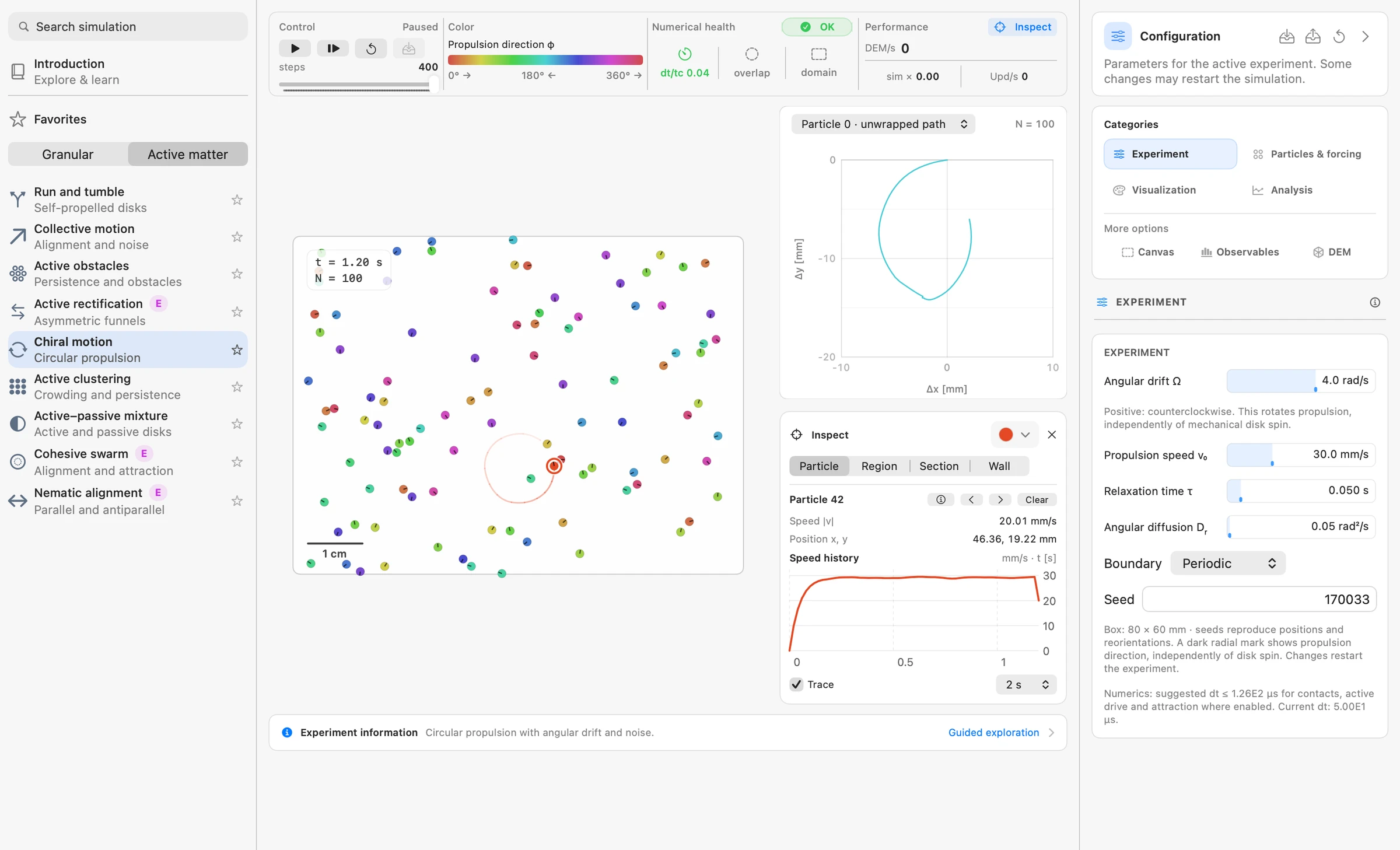
Local analysis
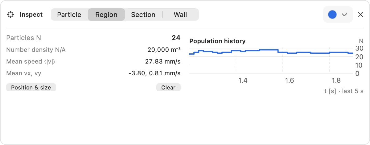
Inspect addresses a selected object or part of space. Its four instruments answer complementary questions.
| Instrument | What to select | What to read |
|---|---|---|
| Particle | One grain | Identity, position, speed, trajectory and available contacts. |
| Region | A fixed rectangle | Particle count, number density and mean motion. |
| Section | An oriented line | Crossings in both directions and net particle flow. |
| Wall | A physical boundary | Available contact reactions and load histories. |
Particle, Region and Wall histories use acquired simulation frames. Section crossings are counted during DEM stepping. A history does not reconstruct values between acquired samples, and periodic edges are not physical walls.
Global analysis
Analysis examines spatial organization across the active system. Availability depends on the experiment.
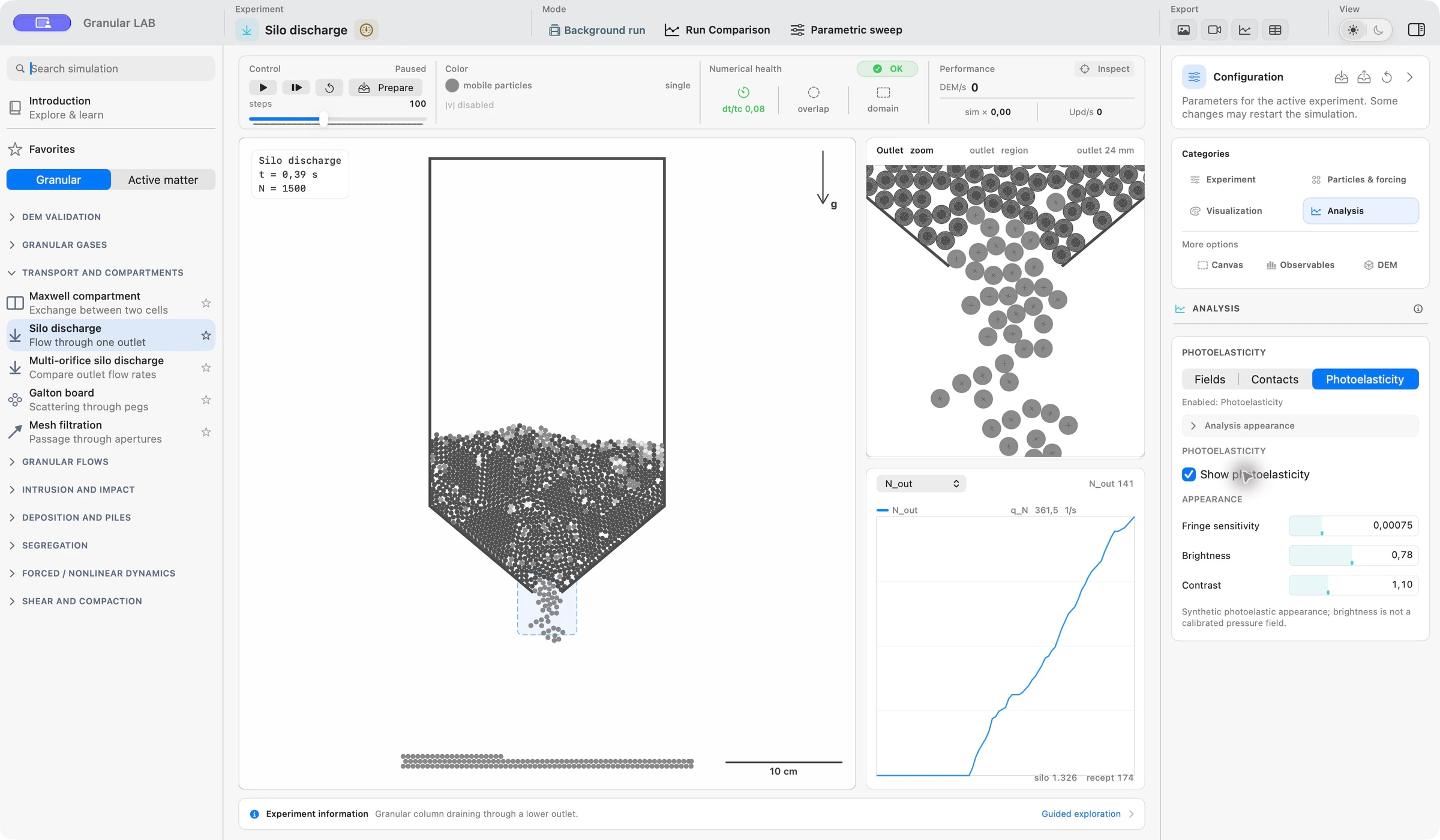
Fields
Map area fraction, mean velocity, speed or agitation. The averaging radius defines a physical measurement scale; grid resolution alone cannot recover detail removed by smoothing.
Contact
Explore contact geometry, spatial order, connectivity and available network descriptors. Contact arrangement and contact load are different quantities.
Force Links
Overlay force links and chains to identify the paths carrying load. Choose thresholds and force scales consistently when comparing states.
Photoelasticity
Visualize a synthetic fringe response to the simulated contact state. Gain and appearance controls change the image, not the mechanical forces. These images are not calibrated photographs of a photoelastic material.
Choose a way to run
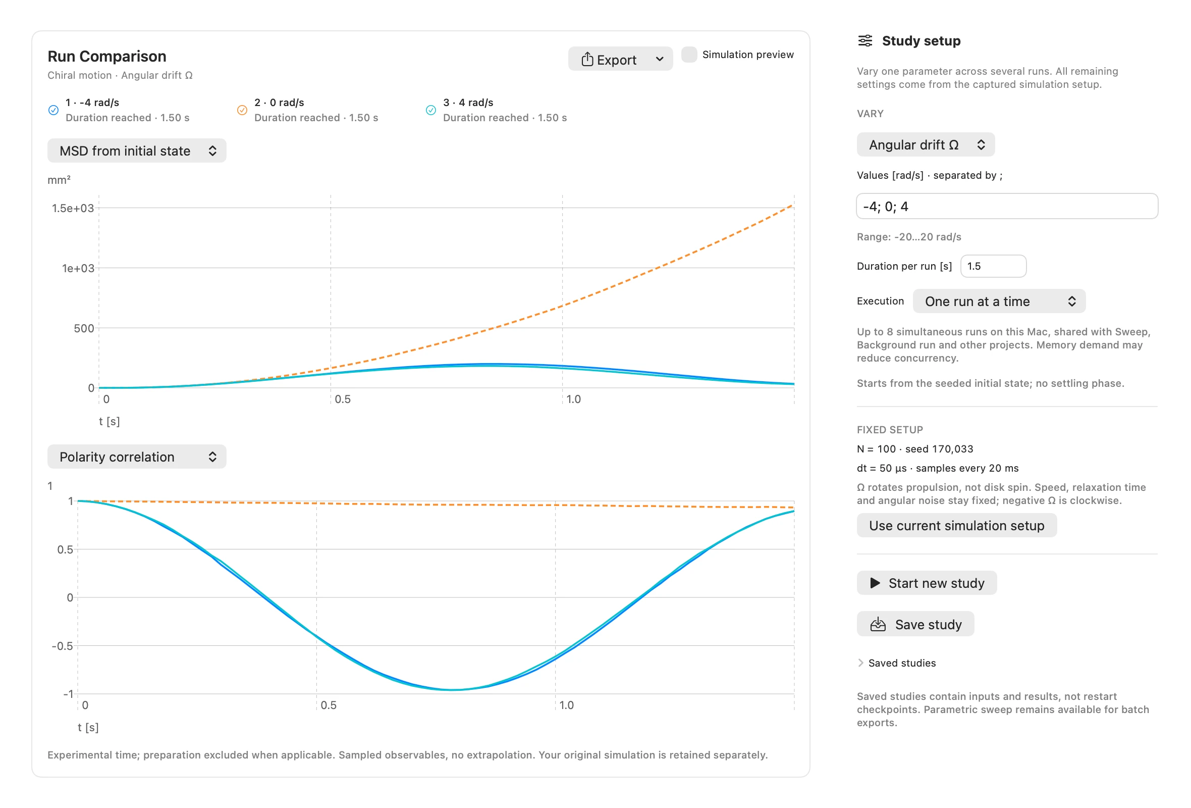
Run Comparison
Vary one parameter across independently evolved runs, read acquired curves on shared axes and export the study. Available in 28 presets, with observables specific to the selected experiment.
Parametric sweep
Explore a parameter range as a batch and retain numerical outputs. Available in 42 presets. The execution settings let compatible cases share the available computing capacity.
Background run
Prepare a separate simulation and choose supported video and data outputs. The interactive workspace remains independent. Keep the complete result folder to revisit supported playback and synchronized observables.
Up to eight independent jobs can run concurrently, depending on CPU and memory. Four or fewer are recommended initially. This is parallel execution of separate simulations, not a claim that a single contact calculation uses every core.
Projects & recorded explorations
A .glab project brings together a captured configuration, instruments, studies, acquired recordings and notes.
- Choose File → New Project from Workspace to capture a supported setup, or use File → Record Exploration to acquire particle frames and selected measurements.
- Review the setup, sampling and notes. Save the project with File → Save.
- Reopen it from Finder or File → Open to consult the saved studies and acquired frames.
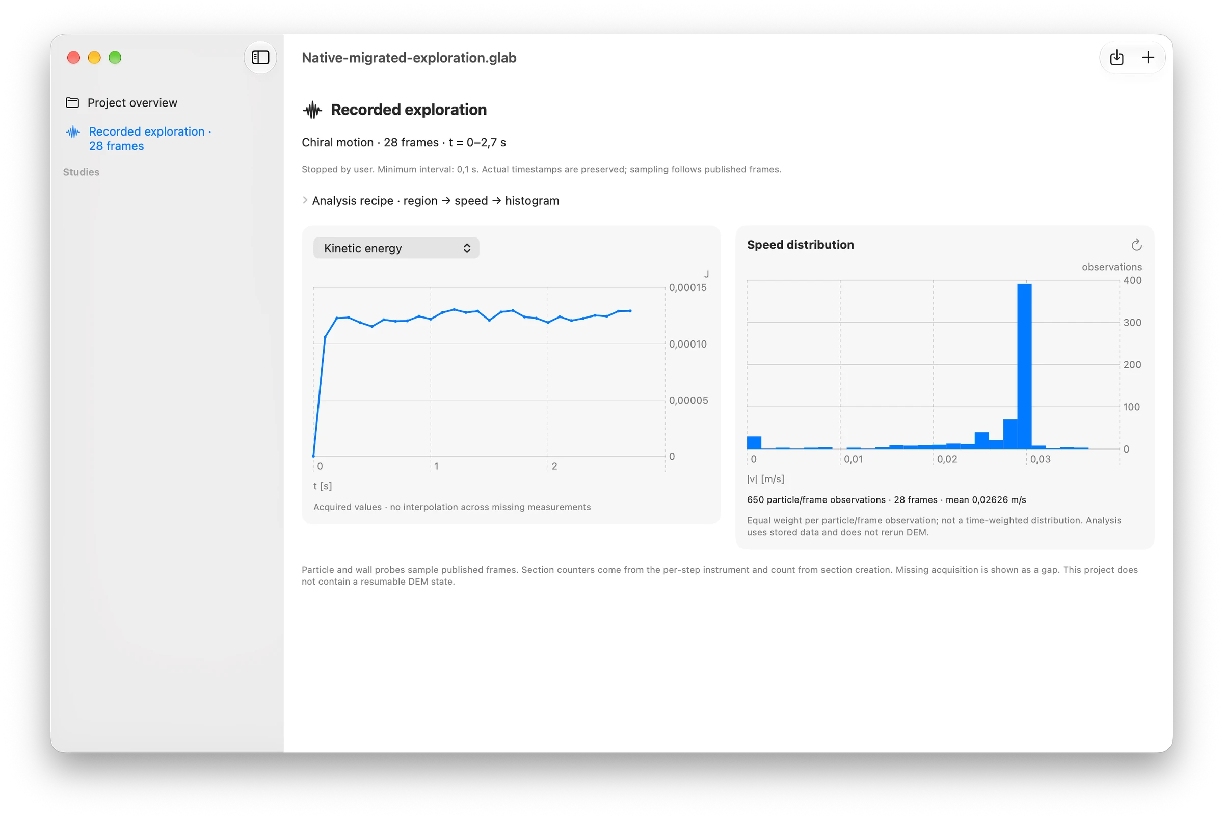
Recorded exploration supports a region → speed → histogram recipe. It does not reproduce every live Analysis layer or restore unsampled motion.
Recording is bounded at 1,200 frames or 200,000 particle states. Projects are limited to 256 MiB, including their index, and 64 studies. A project is not a general physical restart checkpoint. Keep a separate backup of important work.
Export & reproduce
| Output | Use it for |
|---|---|
| Image / PNG | The supported current simulation view. |
| Particle snapshot CSV | Particle properties at one instant. |
| Time series CSV | Acquisition from the current state onward, rather than a retrospective dump of the screen history. |
| Field CSV | Available spatial fields, with coordinates and averaging context. |
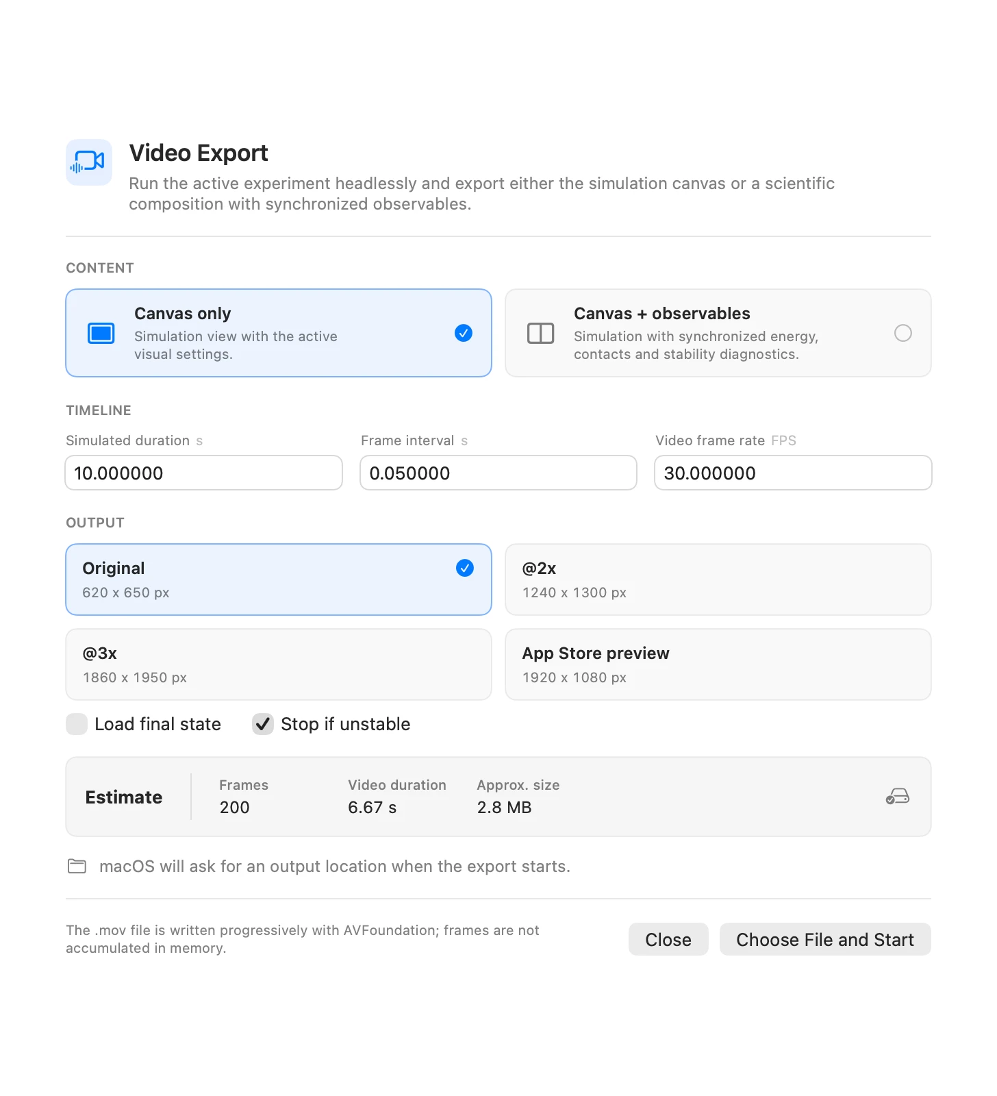
| Video | Supported simulation output; distinguish physical duration from movie playback duration. |
| Comparison export | Study inputs, acquired data and diagnostics, with optional charts. |
| .glab project | Native review of a setup and its acquired work. |
Keep the preset, seed, time step, preparation protocol, units and sampling definition with a quantitative result. Check numerical health and time-step sensitivity before drawing conclusions.
The model behind the motion
In Experiment → Physics of this experiment, read the equations of motion, parameter meanings, units and assumptions for each preset. The app distinguishes the integrated model from relations used to interpret the observations.
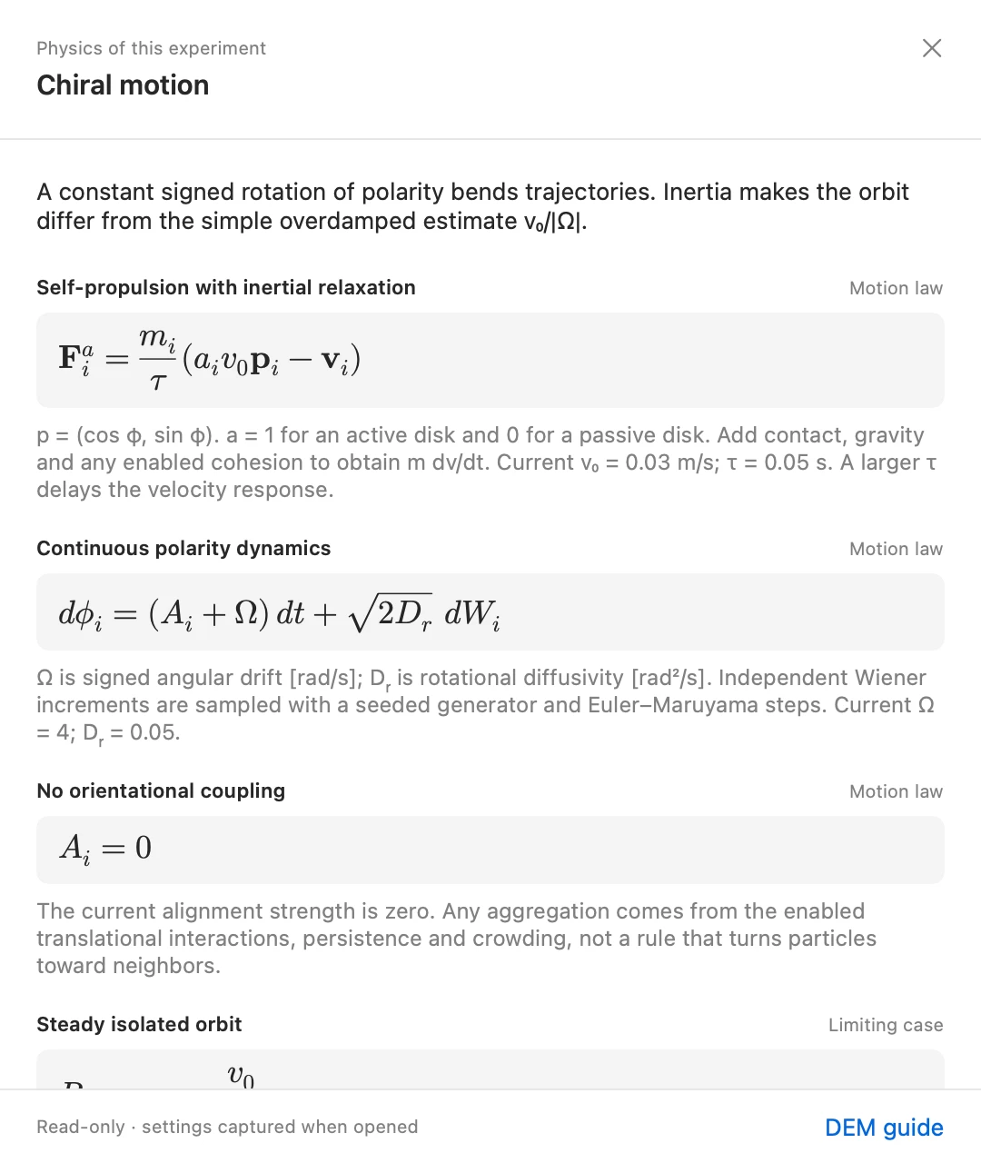
Most experiments use dry soft-particle DEM in two dimensions, with dissipative contacts, friction and rotation where applicable. Selected quasi-2D experiments use 3D spheres, and active-matter presets use idealized propulsion and interaction models.
Read each preset’s scope and maturity. “Implemented” does not mean calibrated in every regime; “Experimental” indicates specific outstanding physical checks. Granular LAB is not a CFD solver or a calibrated biological model.
The complete user manual
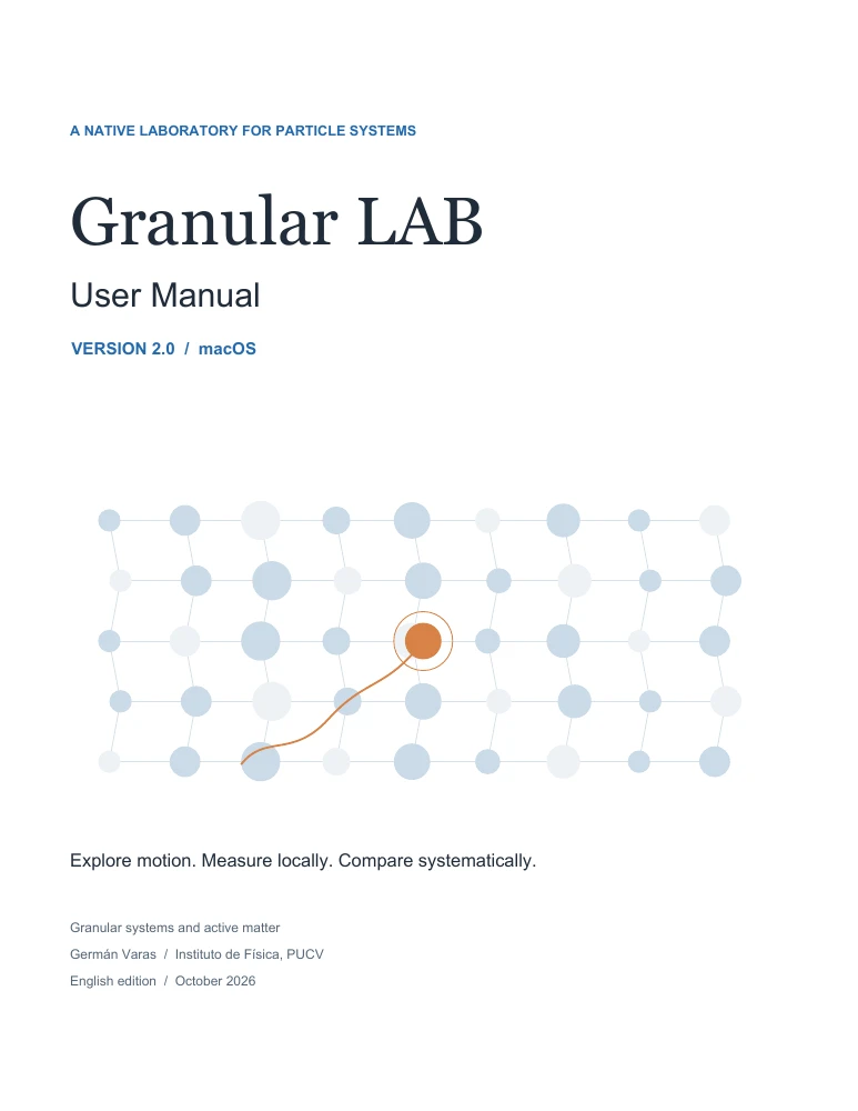
The English PDF covers the workspace, instruments, global analysis, experiments, projects, exports and models, with real app screenshots and a reference for all 47 presets.
Open the Granular LAB 2.0 User Manual (PDF)
The same manual is available offline in the app through Help → User Manual (PDF).