
Find a physical question.
47 experiments, from grain-scale interactions to collective behavior. Choose a family or search for a phenomenon, parameter or observable.
Open an experiment to read its scope. “Experimental” and “In development” identify documented model limitations; an implemented preset is not a validation of every parameter regime.
No matching experiments. Try another term or select all families and tools.
DEM validation
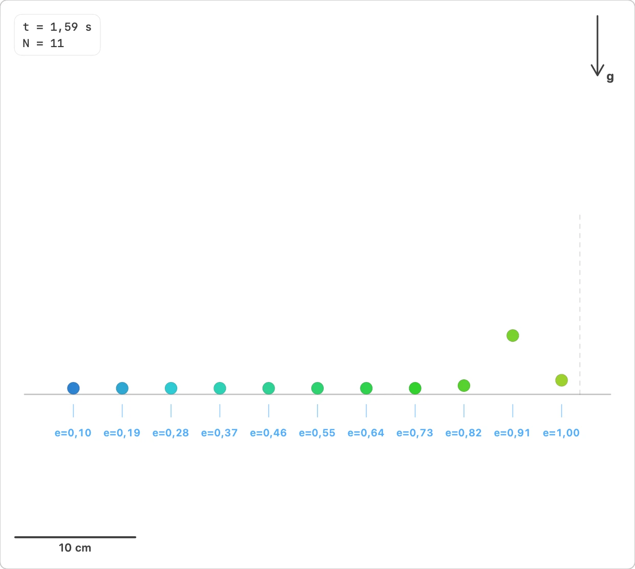
Normal restitution testValidated
How does the first rebound height follow the effective normal restitution measured in a particle-wall impact?
This preset compares nominal and effective normal restitution. The measured rebound height follows h1/h0 ≈ e_eff², where e_eff is obtained from the velocity ratio before and after the first impact. For strongly dissipative impacts, e_eff may differ from the target value because of the discrete soft-sphere contact implementation.
- Parameters:
- Number of particles N · Mean diameter d · Initial free height h0 · Restitution range e_min...e_max · Horizontal spacing · 2D density ρ · Gravity g
- Observables:
- Particle height y_i(t) · Running maximum height h_max,i(t) · First rebound height h1 · h1/h0 vs e_target^2 · h1/h0 vs e_eff^2 · e_eff vs e_target · Estimated restitution sqrt(h1/h0)
- Study tools:
- Run Comparison not available · Parametric sweep
Model & numerical notes
- h0 is the free height between the disk bottom and the base, not the center coordinate.
- e_eff is measured from the vertical velocity ratio before and after the first base impact.
- Particles are spaced horizontally to avoid particle-particle collisions in the reference setup.
- The DEM contact law is unchanged; only gammaN is selected per particle for particle-base contacts.
- For low target restitution, the discrete linear soft-sphere contact can produce an effective restitution above the nominal value.
- e_n = 1 is accepted in the UI and metadata, while the contact-model helper applies its existing numerical clamp internally.
- Monitor maximum overlap and dt/tc when increasing stiffness or gravity.
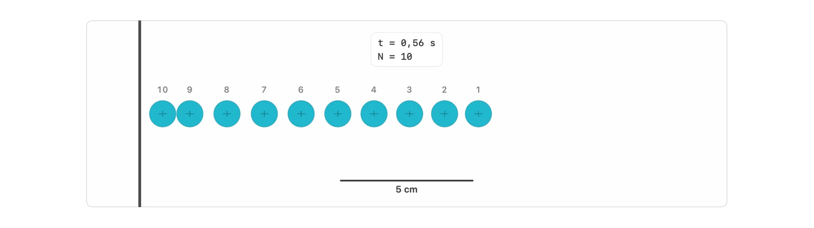
Inelastic chain
How does an impulse travel to a wall and return through a dissipative chain?
A collinear system isolates momentum transfer, restitution and repeated impacts. Choose one-wall impact or a seeded cooling gas between two walls. There is no gravity, friction or background drag. Two lower plots offer trajectories, energy, cumulative collisions and a number-density histogram. Restitution applies to isolated impacts; simultaneous contacts remain genuine DEM dynamics.
- Parameters:
- Particle count N · Diameter d and surface density ρ · Surface gaps / d · Initial speed v0 · Particle restitution e and wall restitution e_w · Normal stiffness k_n and steps per contact
- Observables:
- Trajectories x_i(t) · Velocities v_i(t) · Kinetic and contact energy / E0 · Energy deficit (E0 − K − U) / E0 · Momentum P_x / (m v0) · Cumulative contact episodes C(t): total, pairs, walls · Number density n(x), particles per metre
- Study tools:
- Run Comparison not available · Parametric sweep
Model & numerical notes
- Label i corresponds to particle ID i − 1; label 1 is the rightmost striker. Internal units are SI and mass is ρπd²/4 (2D disks).
- The repulsive linear spring-dashpot force is unchanged. Damping is calibrated separately with reduced mass m/2 for pairs and m for the wall.
- Changing a physical parameter rebuilds the chain and pauses it. No settling stage consumes the initial impulse.
- For p=(1+e)/2 and q=(1−e)/2, the instantaneous two-pass approximation is v1/v0 = e_w p^[2(N−1)] − q² Σ[k=0...N−2] p^(2k). It assumes a specified sequence of binary collisions, not arbitrary recollisions.
- Its sign is not an exact collapse criterion. A finite-duration DEM contact does not reproduce an infinite number of instantaneous collisions in finite time.
- The time window defaults to 3 s and can be set from 0.5 to 30 s without resetting dynamics. Large systems display 30 representative trajectories; all particles remain in the CSV.
- Density uses fixed bins of particle centres over the initial observation interval. Its integral is the in-range particle count; escaped particles are reported separately. This is 1D number density, not material density.
- McNamara & Young Fig. 3 uses instantaneous impacts, e=0.8 and N=14–16. The paper reports about 12500 collisions for N=15. Finite-duration DEM contacts and simultaneous contacts regularize that limit; reducing dt does not remove finite stiffness.
- Their Fig. 8 concerns a different protocol: N=1000 point particles cooling between two walls. Our cooling mode uses finite disks, random non-overlapping positions, centred random velocities and prescribed RMS speed. It is a related experiment, not an exact reproduction of that figure.
- Check overlap and timestep convergence. The energy deficit includes numerical error; temporary spring energy is displayed separately. Collision totals update at every DEM step, independently of screen and export sampling. Sustained positive overlap counts once until separation.
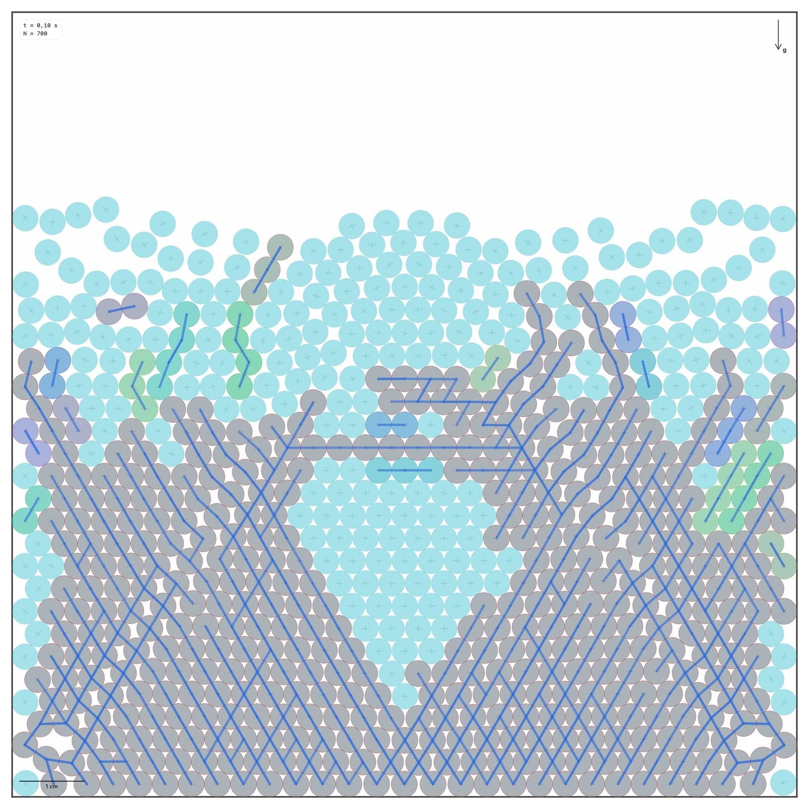
Topology and force networks
How do local order, coordination defects and force-network structure coexist in a 2D granular packing?
This preset presents one DEM packing through six synchronized structural views: a clean system view, contacts or force network, spatial order, and three independently selectable node-metric panels. The force-network panels use particle-particle contacts only; strong components remain the default domain method, while communities and betweenness are exploratory opt-in diagnostics.
- Parameters:
- Particles N · Mean diameter d · Polydispersity · Packing orientation · Initial noise · Gravity g
- Observables:
- Mean coordination · Number of particles with Z=5 · Number of particles with Z=6 · Number of particles with Z=7 · Defect fraction · Boundary particles · Mean |psi6| · Standard deviation of |psi6| · Force-network mean degree · Force heterogeneity · Strong-force domain count · Community count and modularity Q when communities are enabled · Voronoi cells · Approximate Delaunay-like neighbor network
- Study tools:
- Run Comparison not available · Parametric sweep
Model & numerical notes
- Boundary particles have fewer neighbors and are excluded from structural averages.
- |psi6| is computed from an approximate cutoff-based near-neighbor network; it is not an exact Delaunay triangulation or a full KTHNY classification.
- Force-network diagnostics use particle-particle contacts as weighted edges. Wall contacts remain excluded from V1/V2 network analysis.
- The default dashboard enables lightweight strong-force contacts and domains; communities and betweenness remain off until selected.
- For polydisperse particles, classical Voronoi may be insufficient; radical Voronoi remains a future improvement.
- Gravity is enabled by default so the packing rests on the container base.
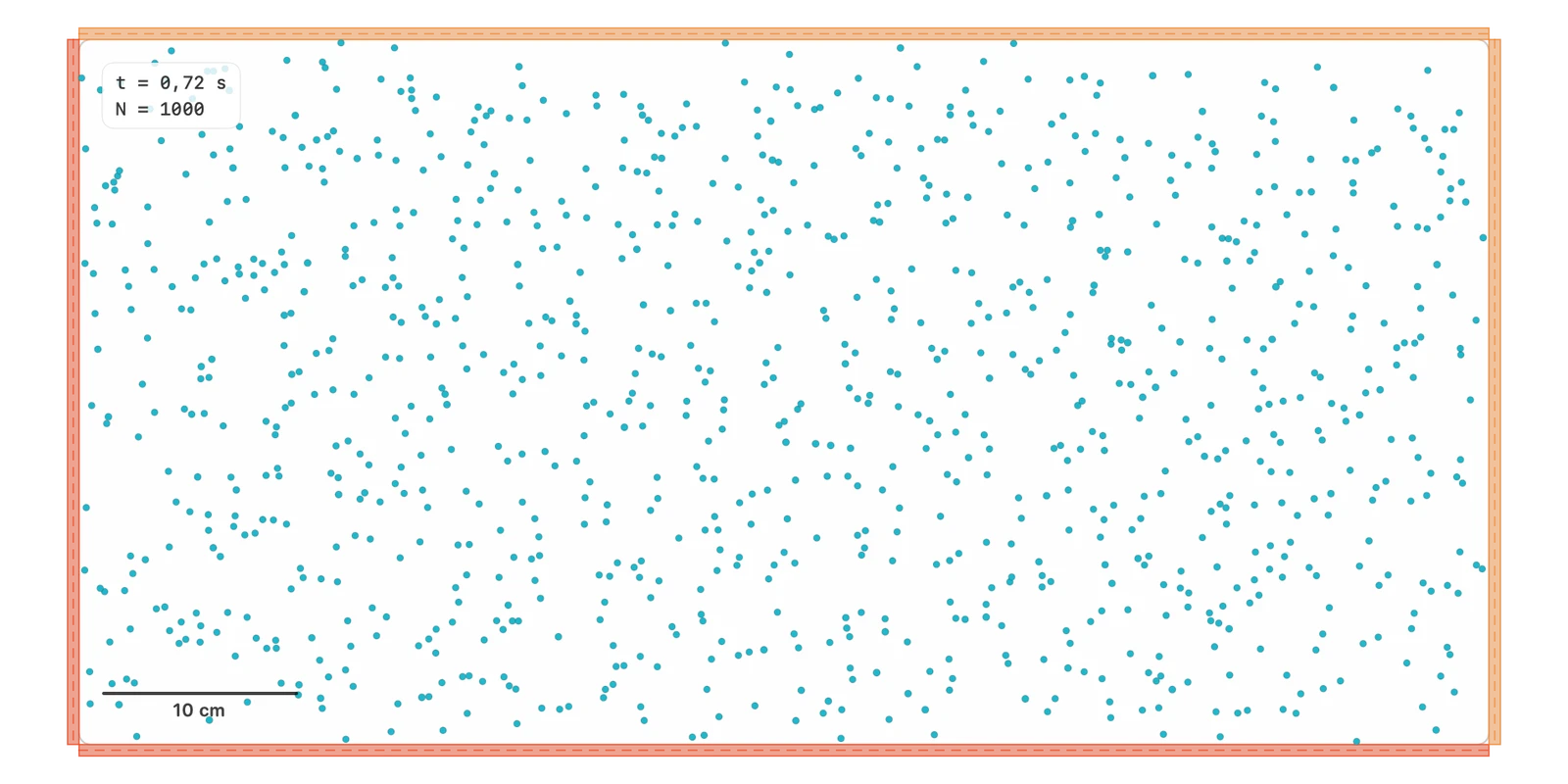
Granular gases
Thermal box
How does a dissipative granular gas reach a steady state when energy is supplied by thermal walls?
Confined two-dimensional granular gas. The walls reinject energy and partially compensate dissipation from inelastic collisions. The velocity distribution may deviate from a Maxwellian because of dissipation, density and the energy-injection mechanism.
- Parameters:
- Particles N · Mean diameter d · Size dispersion · Thermal-wall speed · Friction μ · Damping γ_n/γ_t · Color scale
- Observables:
- T_g · Total kinetic energy · P(|v|) · P(vx) · P(vy) · Contacts · Tx/Ty anisotropy
- Study tools:
- Run Comparison · Parametric sweep
Model & numerical notes
- Avoid initial overlaps.
- Monitor delta max/R.
- Throttle histogram updates.
Periodic gas
How stable is the mechanical energy of a nearly elastic granular gas without walls?
Granular gas in a periodic domain. Removing walls and external sources makes the experiment a test of approximate conservation and numerical integrator stability.
- Parameters:
- Particles N · Area density · Normal restitution e_n / damping γ_n · Friction μ · Step dt · Periodic condition
- Observables:
- Total energy · Contact energy · T_g · P(|v|) · Contacts · delta max/R
- Study tools:
- Run Comparison · Parametric sweep
Model & numerical notes
- Systematic energy growth should not appear without a physical source.
- Use this preset as a control for integrator and contact changes.
- Gravitational potential energy is zero when gravity is absent.
Free cooling
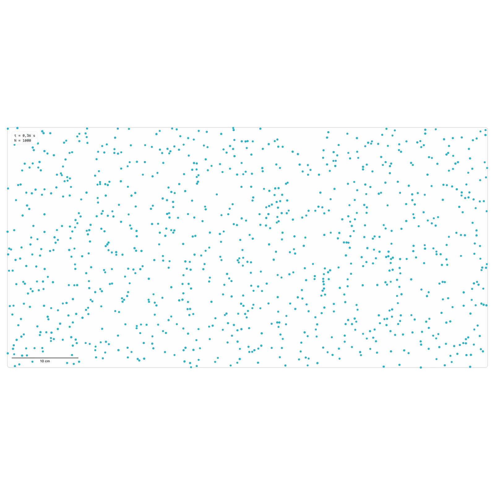
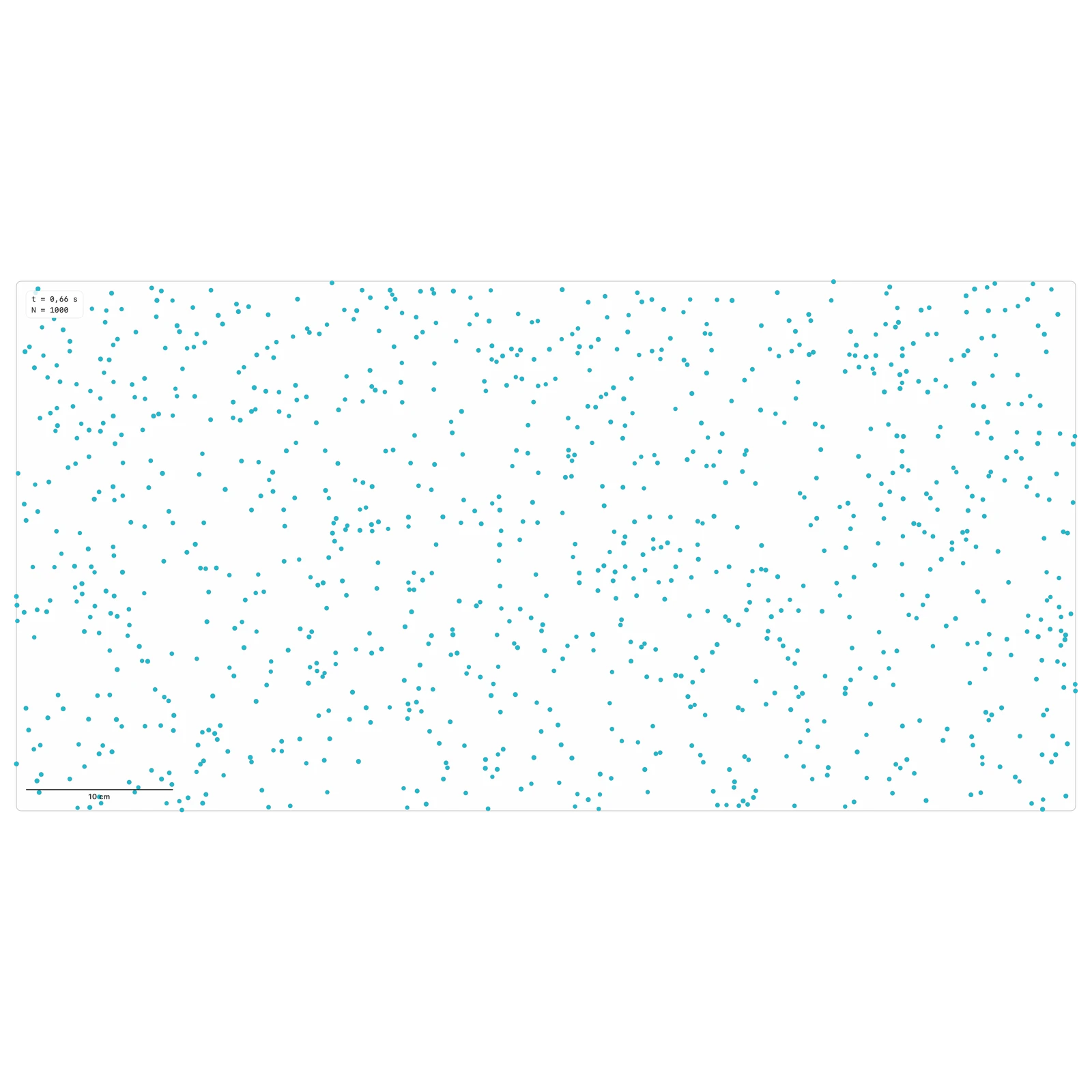
How does granular temperature decay when a dissipative gas receives no external energy?
Free cooling in a periodic domain. The system loses energy through inelastic collisions and shows collective cooling without wall effects.
- Parameters:
- Particles N · Initial density · Normal damping γ_n · Friction μ · Step dt · Periodic condition
- Observables:
- T_g(t) · E_tot(t) · Contacts · P(|v|) · delta max/R
- Study tools:
- Run Comparison · Parametric sweep
Model & numerical notes
- Energy should decay when dissipation is present.
- Avoid an overly dense initial packing.
- Compare dt/tc before interpreting cooling rates.
Fluidized instabilityIn development
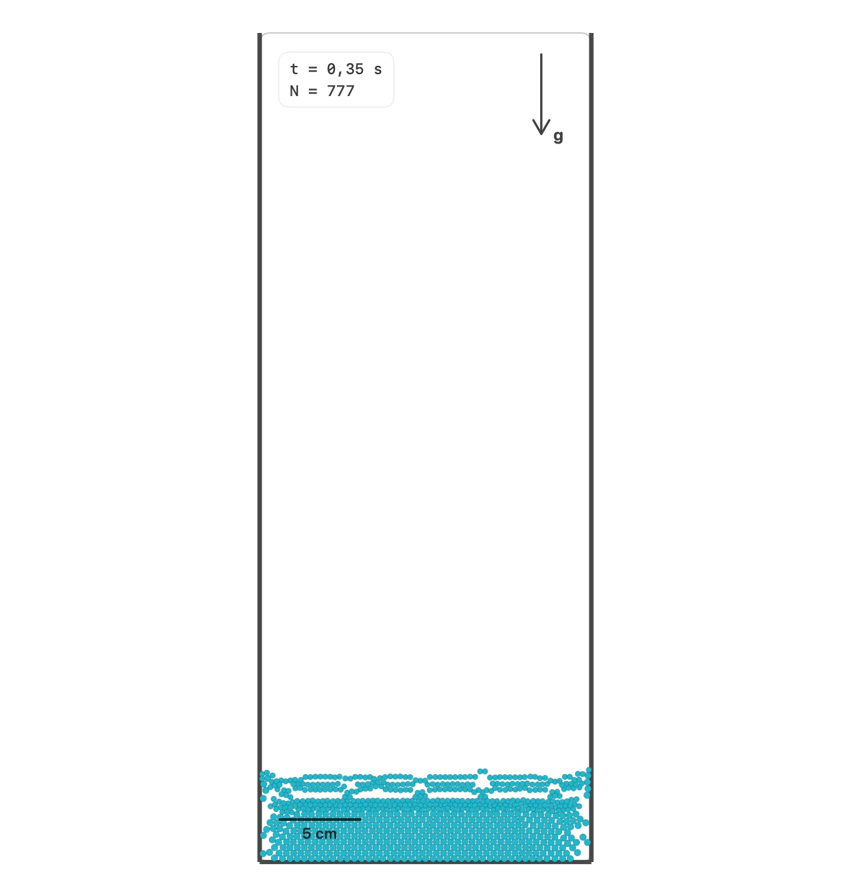
How can upward gas flow, contacts and binary stratification be explored qualitatively?
This preset preserves the experimental GasGrid2D, permeability-channeling and pressureSOR infrastructure for future exploration. It should not be interpreted as a validated reproduction of McLaren et al. 2019 or as full CFD; Granular LAB's immediate priority remains robust DEM presets.
- Parameters:
- N_L and N_H · d_L and d_H/d_L · rho_H/rho_L · U/Umf_L · Vibration Gamma · GasGrid resolution
- Observables:
- Interface A(t) · Dominant lambda · channeling · F_gas/W by species · overlap and dt/tc
- Study tools:
- Run Comparison not available · Parametric sweep not available
Model & numerical notes
- Paused experimental-development preset; keep results as qualitative diagnostics only.
- The gas is porous/coarse-grained: it does not resolve turbulence or bubbles.
- The ug,z velocity is row-normalized and clamped to avoid numerical jets.
- With U = 0, the external gas force should vanish for stationary particles.
Active matter
Run and tumble
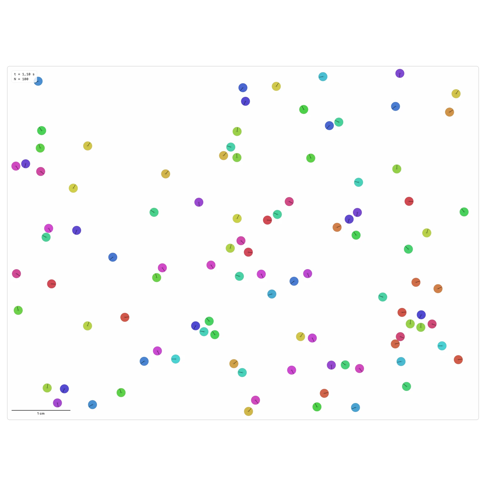
How does persistence change the motion of self-propelled disks?
An inertial run-and-tumble model: m dv/dt = F_contact + m(v₀ p − v)/τ. Polarity p resets to a uniform random angle at Poisson-distributed times. It is independent of mechanical disk rotation.
- Parameters:
- Propulsion speed v₀ [m/s] · Relaxation time τ [s] · Tumble rate λ [1/s] · Particles N, diameter d, box size · Seed
- Observables:
- Single-origin ensemble MSD [m²] · Polarity correlation Cₚ(t) · Mean speed [m/s] · Particle 0 unwrapped trajectory
- Study tools:
- Run Comparison · Parametric sweep
Model & numerical notes
- No thermal noise, aligning torque or hydrodynamic interactions. This is not an overdamped bacterial model.
- Changing a parameter resets the experiment. Reuse the seed for comparisons.
- Use dt ≤ 0.02 min(τ, 1/λ) as well as the contact-time limit; compare with dt/2.
- MSD includes startup and collective drift; do not infer a diffusion coefficient from the initial transient.
- Checked scope: inertial relaxation, Poisson reorientation, free-particle MSD, timestep refinement and periodic/closed operation. This does not calibrate a biological swimmer.
Collective motion
When does local alignment produce collective motion?
Inertial active disks with DEM contacts: m dv/dt = F_contact + m(v₀ p − v)/τ. Polarity follows dφᵢ = κ ⟨sin(φⱼ − φᵢ)⟩ dt + √(2Dᵣ) dWᵢ, averaging other centers within R. All orientations update simultaneously. An isolated disk undergoes angular diffusion without alignment.
- Parameters:
- Propulsion speed v₀ [m/s] and relaxation τ [s] · Alignment κ [1/s] · Perception radius R [m] · Angular diffusion Dᵣ [rad²/s] · Particle count, diameter and seed
- Observables:
- Polarity order |⟨p⟩| · Velocity order |Σv|/Σ|v| · Mean speed · Orientation color and unwrapped trajectory
- Study tools:
- Run Comparison · Parametric sweep
Model & numerical notes
- Vicsek-inspired alignment with inertia and soft contacts, not the classical fixed-speed Vicsek model. No attraction, fluid coupling or biological calibration.
- The perception search is separate from contact detection and uses periodic minimum-image distances. R is a center-to-center distance, independent of diameter.
- Euler–Maruyama polarity updates; dt ≤ 0.02 min(τ, 1/κ, 1/Dᵣ), ignoring zero rates, plus the contact limit. Compare statistical results across seeds and with dt/2.
- Velocity order is speed-weighted and defined as zero at rest. High polarity order does not guarantee high speed or a cohesive flock.
- Checked scope: local polar alignment and angular noise in inertial disks, independent order measurements and low/high-noise controls. High-noise P meets both refinement margins over 24 s across 12 seeds. Six N=400 runs characterize finite-time order; they do not establish a stationary phase or a critical point.
Active obstacles
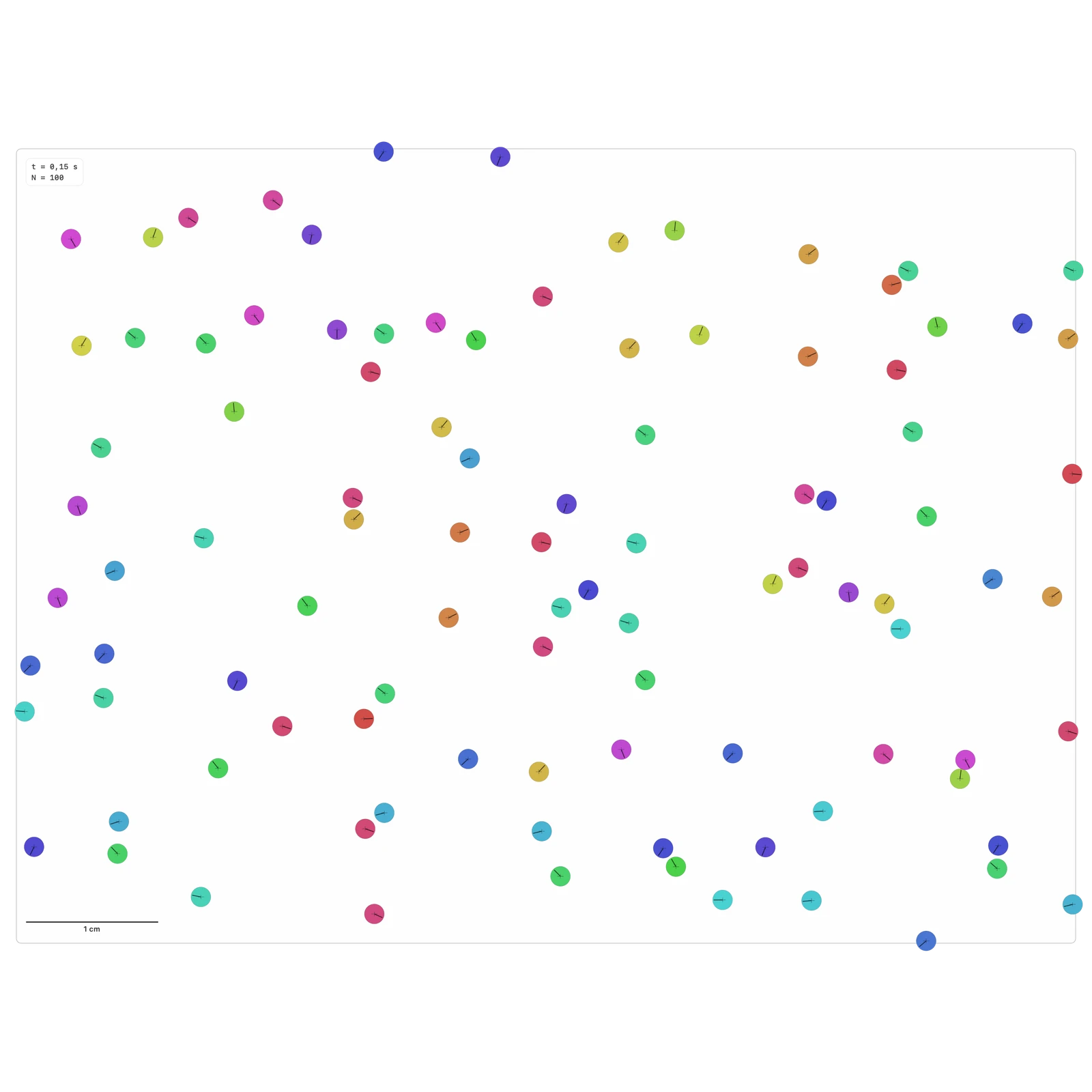
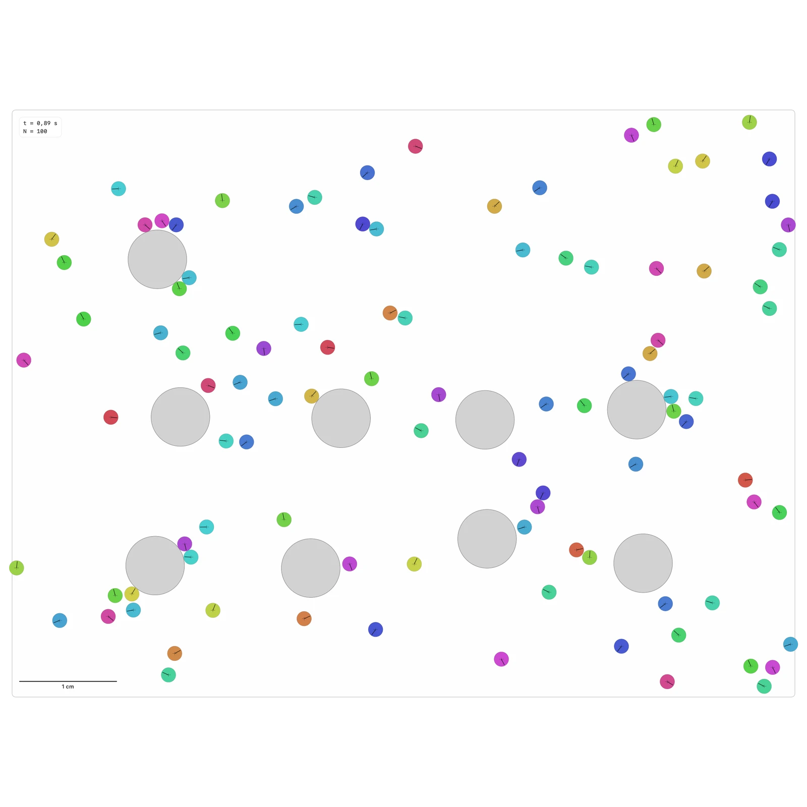
How do obstacles slow and redirect persistent motion?
Dry inertial disks with run-and-tumble propulsion and repulsive DEM contacts. The default box is periodic in both directions; internal obstacles and funnels repeat with it. Contacts change velocity without resetting propulsion direction. A closed box is optional.
- Parameters:
- Single, regular or disordered obstacles · Obstacle count, diameter and geometry seed · Propulsion speed, relaxation time and tumble rate · Particles N, diameter and motion seed
- Observables:
- MSD from initial state · Mean speed · Particle 0 path · Contacts and overlap
- Study tools:
- Run Comparison · Parametric sweep
Model & numerical notes
- No fluid solver or bacterial calibration. Default friction is zero so a persistent particle can slide along a wall. Contact laws and the inertial active drive are shared with Run and tumble.
- Initial positions use reproducible, collision-free shuffled hexagonal sites. Geometry and motion have separate seeds. The UI permits up to 400 particles with 1–2 mm diameters.
- Disordered means bounded, seeded offsets from a regular grid, not a Poisson process. MSD uses unwrapped displacement across periodic edges. Selecting a closed box instead can produce long-time saturation.
- Compare layouts at fixed N, diameter and activity. Changing obstacle count or size also changes available area; compare multiple geometry seeds.
- Use the active accuracy bound and DEM contact-time bound. Monitor overlap, finite state and confinement; compare statistical observables when halving dt.
- Checked scope: periodic transport with single, regular and bounded-disordered obstacles; 100 disks, obstacle radii of 3 and 4 mm, populations of 1, 9 and 16 obstacles, 20 s and three timesteps across 12 seeds. Mobility and surface-band occupancy meet the stated refinement margins. Other parameter regimes still require resolution checks.
Active rectificationExperimental
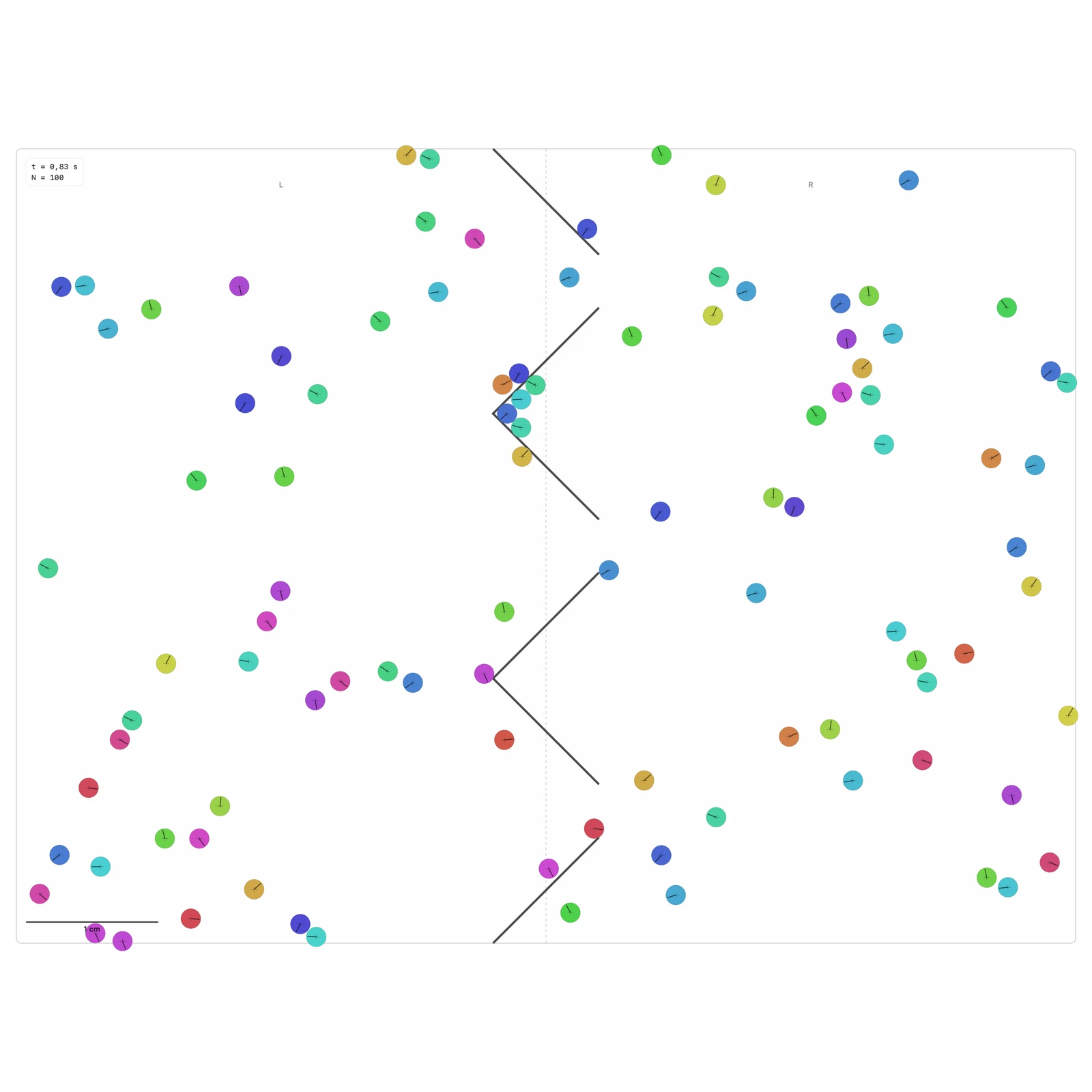
Can asymmetric barriers bias persistent transport?
Dry inertial disks with run-and-tumble propulsion and repulsive DEM contacts. The default box is periodic in both directions; internal obstacles and funnels repeat with it. Contacts change velocity without resetting propulsion direction. A closed box is optional.
- Parameters:
- Funnel direction or symmetric openings · Throat gap, depth and number of funnels · Propulsion speed, relaxation time and tumble rate · Particles N, diameter and motion seed
- Observables:
- Occupancy bias (N_R − N_L)/N · Cumulative L→R and R→L crossings · Net crossings · Mean speed and MSD
- Study tools:
- Run Comparison · Parametric sweep
Model & numerical notes
- No fluid solver or bacterial calibration. Default friction is zero so a persistent particle can slide along a wall. Contact laws and the inertial active drive are shared with Run and tumble.
- Initial positions use reproducible, collision-free shuffled hexagonal sites. Geometry and motion have separate seeds. The UI permits up to 400 particles with 1–2 mm diameters.
- Counts use wrapped particle centers relative to the box midline; equality belongs to R. Every drift counts midline crossings, including recrossings. In a periodic box, ΔN_R = net midline crossings − net positive x-seam crossings; the export includes both counters.
- Periodic boundaries permit repeated transport through the barrier. Occupancy bias alone is not a current: compare the slope of net midline crossings for mirrored funnels and symmetric openings across seeds and dt/2. A closed box supports redistribution, not a permanent net current.
- Use the active accuracy bound and DEM contact-time bound. Monitor overlap, finite state and confinement; compare statistical observables when halving dt.
- Experimental: mirrored funnels reverse transport and the periodic population balance is exact. Two of six occupancy-refinement intervals in the 12-seed, 30 s campaign extend beyond the ±0.05 margin. The symmetric control also needs more statistical precision; the same seeds have a small free-drive drift. This is not a confirmed contact failure, but the acceptance criterion remains open.
Chiral motion
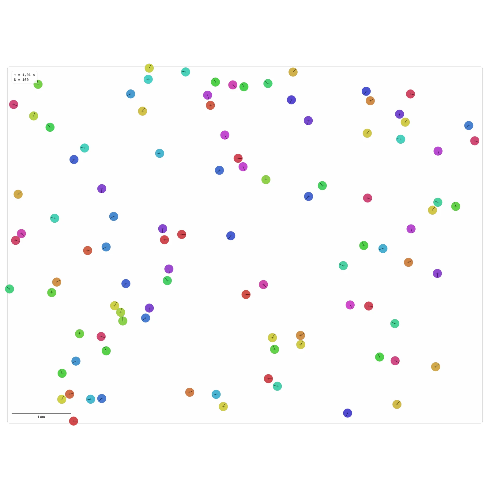
How does rotating propulsion bend a disk's path?
Dry inertial disks with repulsive DEM contacts, linear drag and independently evolving propulsion direction. There is no fluid solver or thermal translational noise.
- Parameters:
- Signed angular drift Ω [rad/s] · Angular diffusion Dᵣ [rad²/s] · Propulsion speed v₀ and relaxation τ · N, diameter and seed
- Observables:
- Particle 0 unwrapped path · Polarity correlation · MSD and mean speed
- Study tools:
- Run Comparison · Parametric sweep
Model & numerical notes
- dφ/dt = Ω + √(2Dᵣ) ξ(t). Positive Ω is counterclockwise. This is propulsion rotation, not mechanical disk spin.
- For one isolated noiseless disk, the inertial steady orbit radius is v₀ / (|Ω| √(1 + Ω²τ²)); v₀/|Ω| is only the small-inertia limit. Ω = 0 restores straight propulsion with relaxation.
- The ensemble polarity reference exp(−Dᵣt) cos(Ωt) applies to independent orientations. Collisions change motion, not polarity.
- Use SI units internally. Orientation uses simultaneous Euler–Maruyama updates. dt obeys active-relaxation, angular-rate and DEM contact limits. Check overlap and finite state; compare dt/2 and several seeds.
- This exploratory finite inertial system does not establish a phase diagram or reproduce a calibrated experimental swimmer. Persistent aggregates alone are not proof of motility-induced phase separation.
- Checked scope: inertial circular motion with positive, negative and zero polarity rotation, noisy correlation, work/drag and boundary operation. Mechanical disk spin is a separate quantity.
Active clustering
Can persistence and crowding create dense groups without attraction?
Dry inertial disks with repulsive DEM contacts, linear drag and independently evolving propulsion direction. There is no fluid solver or thermal translational noise.
- Parameters:
- Nominal area fraction φ · Propulsion speed v₀, relaxation τ and angular diffusion Dᵣ · N, diameter and seed · Cluster distance threshold
- Observables:
- Largest cluster fraction · Particle-weighted cluster size · Spatial number variance / mean · Mean speed
- Study tools:
- Run Comparison · Parametric sweep
Model & numerical notes
- No aligning torque or attractive force. The initializer shuffles a nonoverlapping periodic triangular lattice; let the transient relax before interpreting clusters.
- φ = Nπ(d/2)²/A is nominal, without subtracting overlaps. Box dimensions are fixed. Changing N or diameter changes φ; the displayed value is derived from the actual configuration.
- Groups join centers at distance ≤ threshold × (rᵢ+rⱼ), using minimum images. Weighted size is Σs²/N, including isolated grains. Spatial variance uses a fixed 8×8 grid; it is not a temporal fluctuation measurement.
- Use SI units internally. Orientation uses simultaneous Euler–Maruyama updates. dt obeys active-relaxation, angular-rate and DEM contact limits. Check overlap and finite state; compare dt/2 and several seeds.
- This exploratory finite inertial system does not establish a phase diagram or reproduce a calibrated experimental swimmer. Persistent aggregates alone are not proof of motility-induced phase separation.
- Checked scope: periodic repulsive active disks, independent connectivity measurements and density/noise controls. The dense N=100 case meets the connectivity and speed refinement margins over 24 s across 12 seeds. One-second membership retention permits mergers and is not a cluster lifetime; a large connected group alone does not establish phase separation.
Active–passive mixture
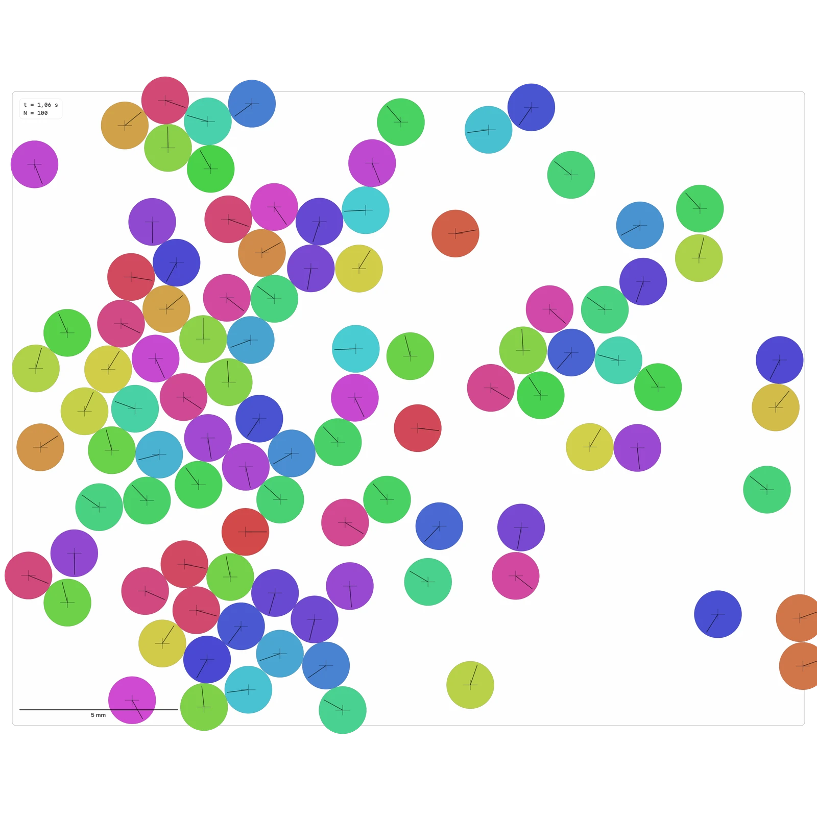
How does an active population transport passive neighbors?
A minimal dry, inertial active-particle model on the shared DEM engine. All quantities use SI internally. There is no CFD, solvent momentum field or calibrated biological response.
- Parameters:
- Active fraction: round(f × N) particles of species A · Total N and derived area fraction φ in a fixed box · Propulsion speed, relaxation and angular diffusion · Diameter and seed
- Observables:
- MSD by activity · Mean speed by activity · Unlike neighbor fraction · Largest cluster fraction
- Study tools:
- Run Comparison · Parametric sweep
Model & numerical notes
- A is propelled; B has zero propulsion. Both have the same mass, diameter, drag and repulsive contacts. Passive disks are athermal: without active collisions they relax to rest.
- Species labels occupy independently shuffled lattice sites. Their fixed IDs, displacement and species survive snapshots. Active and passive mobility use their own population counts. An absent species exports count zero and mobility zero; its plotted series is omitted.
- Unlike neighbor fraction is the number of A–B edges divided by all edges at the cluster distance threshold, with minimum images. It is zero when no edges exist. This is a structural comparison, not a calibrated segregation index.
- Orientations update simultaneously with Euler–Maruyama, independently of mechanical spin. Seeds reproduce the same timestep and configuration; noisy trajectories need not match when dt changes.
- Compare several seeds, system sizes and dt/2. Check overlap, finite state and confinement. A finite cluster or ordered configuration does not establish a phase diagram.
- Checked scope: periodic active/passive disks with equal mass, diameter and drag; passive particles receive motion through contacts. The 50/50, N=100 case meets connectivity and both species-speed refinement margins over 24 s across 12 seeds. Neighbor composition is a geometric measurement, not by itself evidence of segregation.
Cohesive swarmExperimental
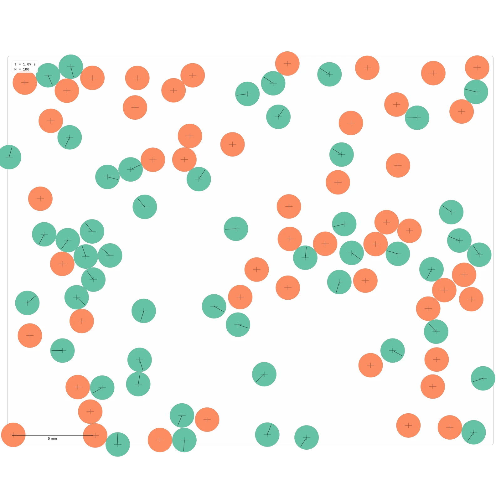
How do attraction and alignment compete with active spreading?
A minimal dry, inertial active-particle model on the shared DEM engine. All quantities use SI internally. There is no CFD, solvent momentum field or calibrated biological response.
- Parameters:
- Maximum attraction F₀ [N] and range / d · Polar alignment κ and perception radius R · N, derived density φ, propulsion and angular diffusion · N, diameter and seed
- Observables:
- Largest cluster fraction · Polarity order · Particle-weighted cluster size · Mean speed
- Study tools:
- Run Comparison · Parametric sweep
Model & numerical notes
- Attraction is central and equal/opposite. For d = rᵢ+rⱼ, ℓ = (rangeFactor−1)d and s = (r−d)/ℓ: F = F₀ sin(πs) towards the neighbor for 0 < s < 1, zero otherwise. Repulsion is ordinary DEM.
- U = −F₀ℓ(1+cos(πs))/π in the attraction range, constant −2F₀ℓ/π below contact and zero beyond cutoff. Force and potential are continuous at both joins. Attraction has a separate sparse neighbor search and does not alter contact history.
- Attraction range, alignment radius and cluster threshold are three independent distances. A bound pair outside the cluster threshold is not counted as a connected group. F₀ = 0 removes attraction but retains alignment.
- The generic mechanical-energy diagnostic omits the added attraction potential. Do not use it alone for energy conservation. Attraction is not included in DEM contact-force chains. A conservative slope-based timestep check supplements the contact and active-drive bounds.
- Orientations update simultaneously with Euler–Maruyama, independently of mechanical spin. Seeds reproduce the same timestep and configuration; noisy trajectories need not match when dt changes.
- Compare several seeds, system sizes and dt/2. Check overlap, finite state and confinement. A finite cluster or ordered configuration does not establish a phase diagram.
- Experimental: pair attraction and energy accounting are checked. In the 12-seed, 12 s reference campaign, polar order and one-second membership retention meet the refinement margin, but both largest-group intervals extend beyond ±0.05. Without attraction, membership-retention precision also remains unresolved. Retention permits mergers and is not a cluster lifetime.
Nematic alignmentExperimental
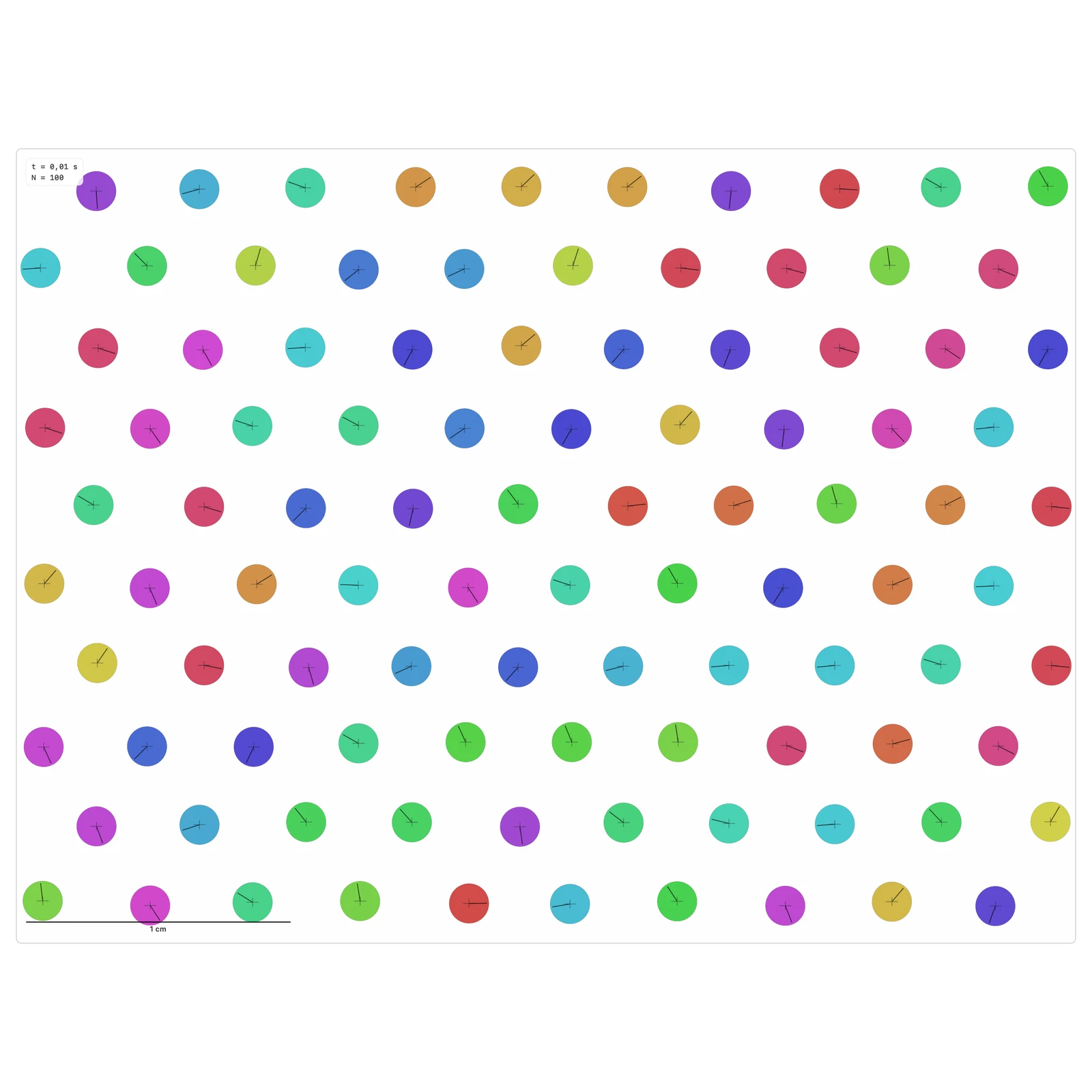
Can orientational order exist without a common direction of travel?
A minimal dry, inertial active-particle model on the shared DEM engine. All quantities use SI internally. There is no CFD, solvent momentum field or calibrated biological response.
- Parameters:
- Alignment κ [1/s] · Perception radius R [m] · Angular diffusion Dᵣ [rad²/s] · Propulsion speed, relaxation, N and seed
- Observables:
- Nematic order S = |⟨exp(2iφ)⟩| · Polarity order P = |⟨exp(iφ)⟩| · Velocity order · MSD
- Study tools:
- Run Comparison · Parametric sweep
Model & numerical notes
- dφᵢ/dt = κ meanⱼ sin(2(φⱼ−φᵢ)) + √(2Dᵣ) ξᵢ. Perception excludes self and uses minimum-image distances within R. κ is not divided by two.
- Parallel and antiparallel headings share a nematic axis. An equally split antiparallel population has S = 1 and P = 0. Each disk still propels along its own polar heading.
- These are circular DEM disks with nematic steering. They are not rods, do not acquire steric rod alignment, and do not model wet active-nematic defects or hydrodynamics. The cited rod experiment motivates the distinction in order, not quantitative agreement.
- Orientations update simultaneously with Euler–Maruyama, independently of mechanical spin. Seeds reproduce the same timestep and configuration; noisy trajectories need not match when dt changes.
- Compare several seeds, system sizes and dt/2. Check overlap, finite state and confinement. A finite cluster or ordered configuration does not establish a phase diagram.
- Experimental: head–tail symmetry and nematic order S are checked. Secondary polar order P varies strongly between seeds; both P refinement intervals remain wider than the ±0.05 acceptance margin in the 12-seed, 24 s campaign. Finite-size ordering and transients must be distinguished from a stationary phase.
Transport and compartments
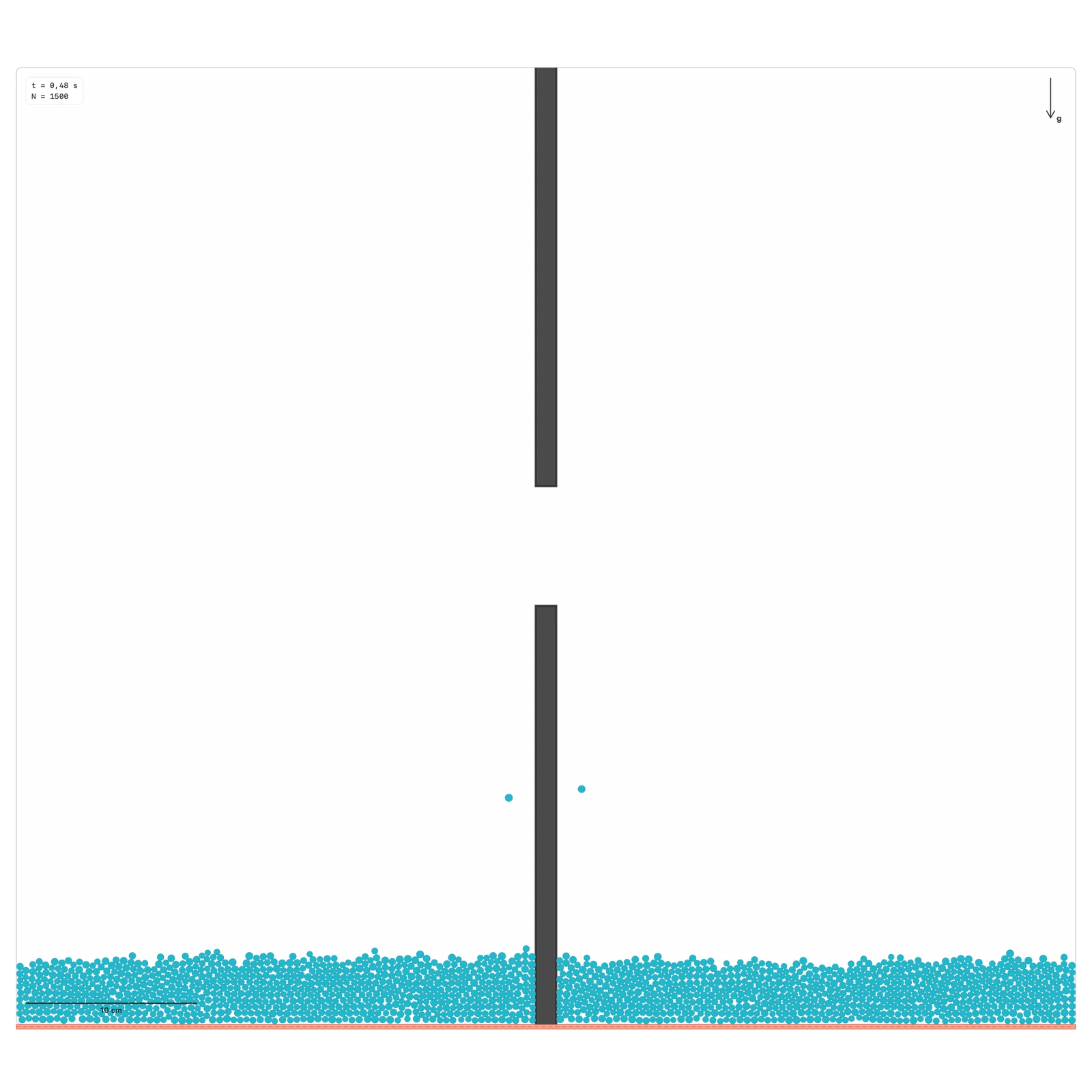
Maxwell compartment
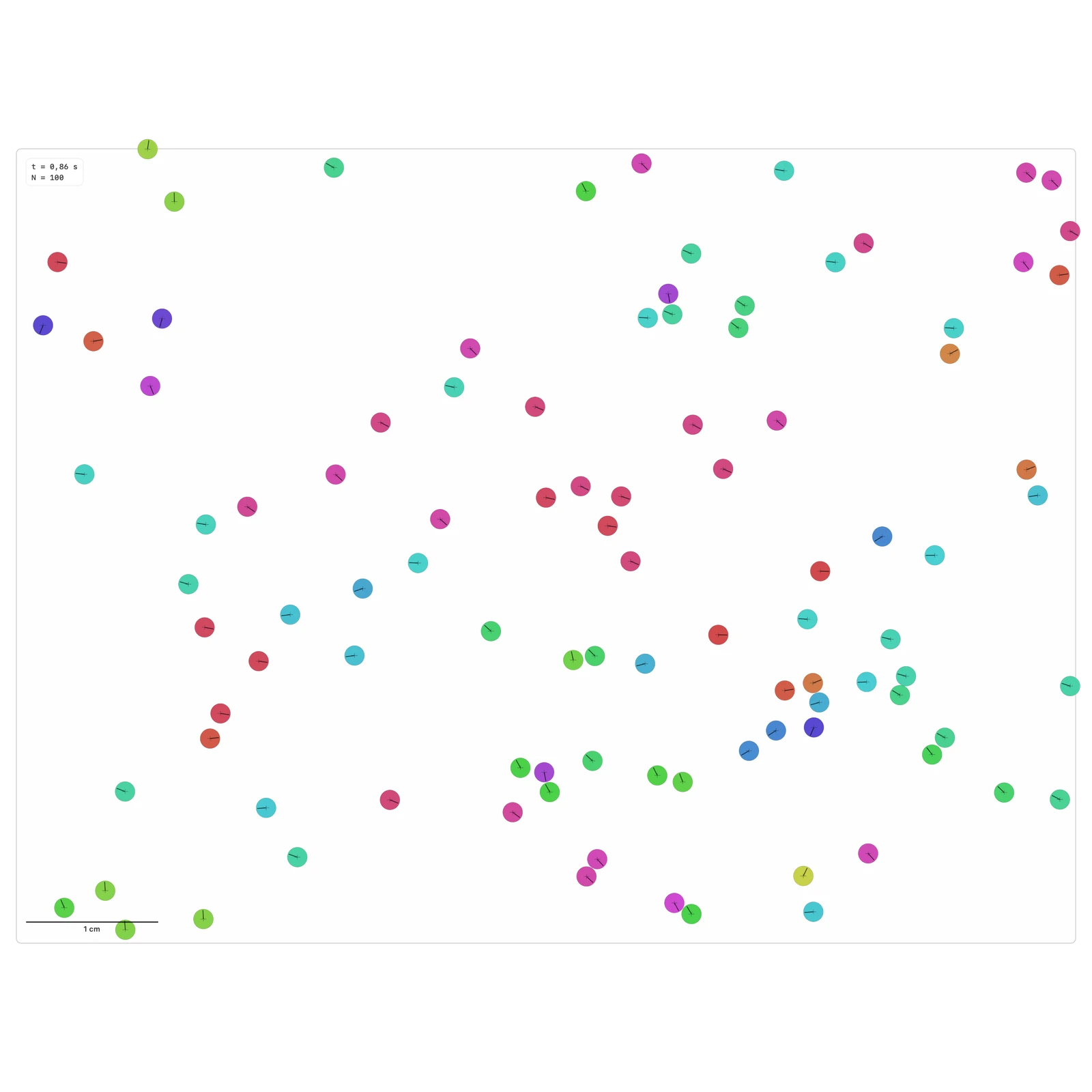
How does the population evolve between two compartments connected by an aperture?
Two cells separated by a wall with a central opening. It supports studying transport, mixing and sensitivity to opening size/position.
- Parameters:
- Particles N · Opening height · Opening position · Gravity g or no gravity · Friction μ · Damping γ_n
- Observables:
- Particles per compartment · Flow through the opening · Energy · Contacts · delta max/R
- Study tools:
- Run Comparison · Parametric sweep
Model & numerical notes
- The wall must repel from both accessible faces.
- Do not seed particles inside the divider.
- Avoid openings so small that they compress particles during rebuild.
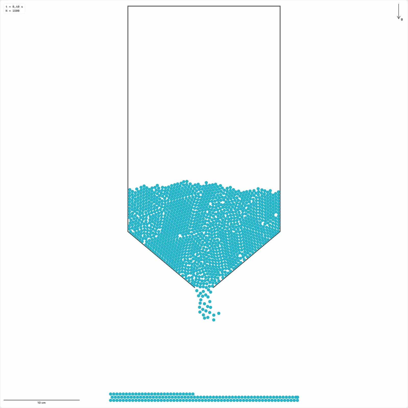
Silo discharge
Why can the discharge rate of a granular silo be approximately constant and independent of column height?
Grain column discharging through a lower opening. The cumulative discharged particle count N_out(t) reveals the steady regime; an approximately linear region indicates a nearly constant particle discharge rate.
- Parameters:
- Particles N · Mean diameter d · Dispersion · Outlet width · Box width · Box height · Bottom angle · Gravity g · Friction μ · Global damping · Silo geometry
- Observables:
- N_out(t) · Particle discharge rate q_N = dN_out/dt · Base load F_base(t) · Lateral load F_lateral(t) and p_lateral,2D(t) · Particles inside the silo · Clogging events
- Study tools:
- Run Comparison · Parametric sweep
Model & numerical notes
- Initialize without severe overlaps.
- Use initial relaxation if needed.
- Avoid particles trapped at the outlet.
- Discharged particles are captured as a diagnostic without drawing a physical receiving container.
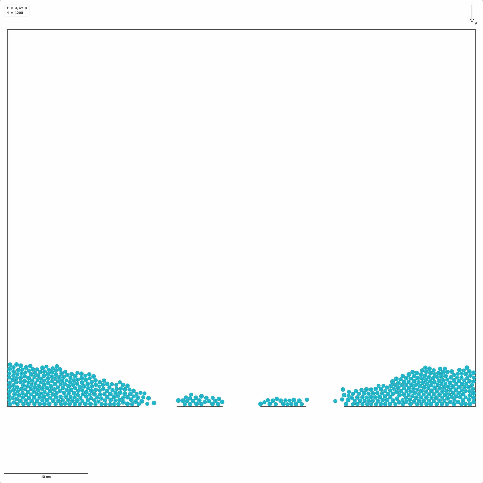
Multi-orifice silo discharge
How does a granular column split its discharge among multiple lower outlets?
Rectangular silo with a flat bottom and several centered orifices. It tracks total discharged mass M_out(t), per-orifice mass M_out,i(t), flow Q_i and outlet balance.
- Parameters:
- Number of orifices n · Mean diameter d · Dispersion · Orifice diameter D · Center spacing s · Box width W · Box height H · Initial fill height H_fill · Gravity g · Friction μ · Global damping
- Observables:
- N_out,total · N_out,i · M_out,total · M_out,i · Q_total · Q_i · Outlet balance · Maximum overlap ratio
- Study tools:
- Run Comparison · Parametric sweep
Model & numerical notes
- Orifices are centered and clamped to fit inside W with a minimum solid ligament.
- Discharged particles are counted only when x falls inside an orifice interval.
- Captured particles are discarded below the visible domain and do not create a lower receptacle.
- Use fixed seeds when comparing outlet balance across layouts.
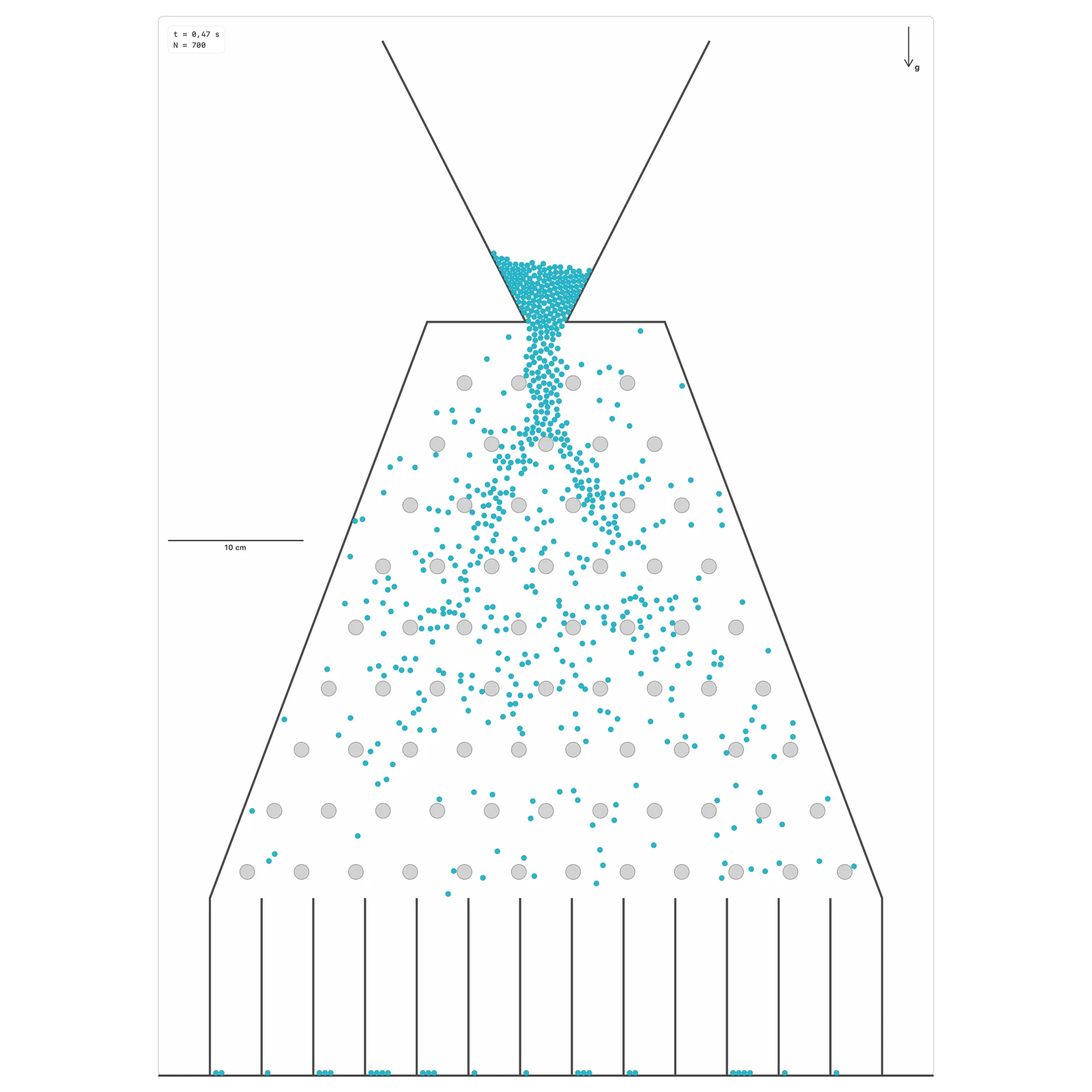
Galton board
How does a lateral outlet distribution emerge when particles fall through a periodic obstacle array?
Disks falling under gravity through a pin array. Each collision changes the trajectory and the ensemble produces an outlet distribution in the lower bins. It supports discussion of diffusion, dispersion and granular mixing.
- Parameters:
- Particles N · Mean diameter d · Pin radius · Horizontal spacing · Vertical spacing · Number of rows · Friction μ · Normal restitution e_n / damping γ_n · Board width · Bin geometry
- Observables:
- Histogram by bin · Lateral outlet distribution · Fall time · Collisions per particle · Particles outside domain · Maximum overlap · Mixing by species when applicable
- Study tools:
- Run Comparison · Parametric sweep
Model & numerical notes
- Avoid overlaps with pins or walls.
- Inject particles gradually.
- Ensure side walls.
- Lower bins must detect particles without generating artificial contacts.
Mesh filtration
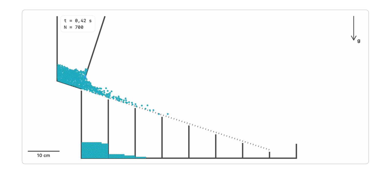
How do filtration and size segregation develop along an inclined mesh?
A grain assembly flows over a perforated inclined mesh. The historical settled-release protocol starts from a column resting on the mesh; funnel feed retains the material between two inclined walls and releases it through a horizontal gate above the solid lead-in. The Particles panel can prepare either one size distribution or a bilayer: species A is placed below species B with independent diameters and a controlled number fraction. The gate height and opening set the initial fall and feeding width before the perforated section. The collector composition then reveals how filtration and segregation depend on the size-to-aperture ratio.
- Parameters:
- Particles N · Initial layering: single size or bilayer · Mean diameter d · Lower/upper diameters d_A and d_B · Lower-layer number fraction · Feed condition · Gate opening G · Funnel opening D_f · Funnel gate height h_f · Aperture D · Ratio chi=d/D · Relative thickness delta/D · Inclination angle · Number of compartments below the perforated zone · Friction μ · Gravity g
- Observables:
- Filtered mass by compartment · Fraction mu_i · Profile mu(x) · Filtration length ell · Remaining survival mass M(x) · Local filtration rate k(x) · Asymptotic rate k_0 and development length x_s · Local filtration length ell_local=1/k_0 versus global ell_fit · Residual mass · Total filtered fraction · Species-filtered fractions F_A and F_B · Species-B fraction by collector x_B,i · Collector segregation index S_bins · Vertical separation S_y of uncollected grains
- Study tools:
- Run Comparison · Parametric sweep
Model & numerical notes
- The mesh is represented with finite segments to avoid invisible walls over apertures.
- Filtered particles are counted once and remain dynamic inside the bins.
- Estimating ell requires enough bins with significant mass; v1 reports ell as n/a.
- M(x) is an empirical survival profile built from classified outcomes: filtration positions and the residual mass reaching the end of the mesh.
- k(x) uses a centered derivative of a smoothed M(x); bins near the edges and below the configured remaining-mass threshold are intentionally omitted.
- k_0 is the median of the trailing valid rate samples, and x_s is the first valid position whose remaining evaluated suffix stays within the configured tolerance around k_0.
- Filtration-specific profiles are derived diagnostics and do not modify the physics.
- S_bins is the total-variation distance between the collected-bin distributions of A and B: 0 means identical distributions and 1 means disjoint distributions.
- S_y=(mean(y_B)-mean(y_A))/H is positive while the uncollected upper species remains above the lower species.
Granular flows
Inclined plane
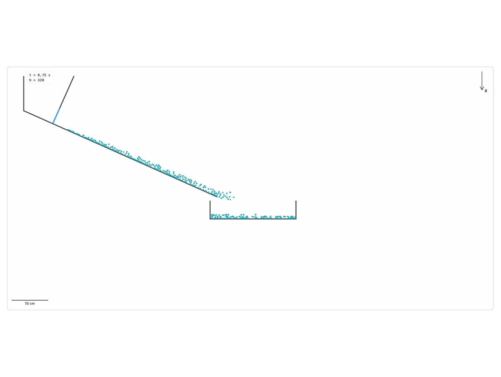
How do inclination and an optional obstacle change a granular release?
A finite sample is prepared behind a hopper gate and released onto a continuous inclined base. Explore angle, friction and gravity, then optionally add one fixed circular obstacle tangent to the plane. Its diameter and centre distance from the start of the plane are adjustable. This two-dimensional cross-section allows grains to pass over the obstacle, without transverse side-wall effects. Contacts use the same grain-boundary DEM model as the base.
- Parameters:
- Particles N · Mean diameter d · Polydispersity · Plane angle · Optional obstacle diameter and position · Grain-grain friction μ · Grain-boundary friction μ · Damping γ_n/γ_t · Gravity g
- Observables:
- Mean velocity parallel to the plane · Center of mass · Parallel displacement · Kinetic energy · Contact count · Maximum overlap
- Study tools:
- Run Comparison · Parametric sweep
Model & numerical notes
- Avoid high initial overlaps between the layer and base.
- The base is continuous. Obstacles is off by default; enabling it adds one fixed disk without adding basal roughness.
- Velocity and displacement average active grains, including those in the hopper; they are not local flow profiles. Base-force plots exclude the obstacle reaction.
- Monitor particles outside the domain at large angles.
- Measure velocities in coordinates parallel/normal to the plane.
- Use Velocity Verlet for dense flow and persistent contacts.
Inclined plow
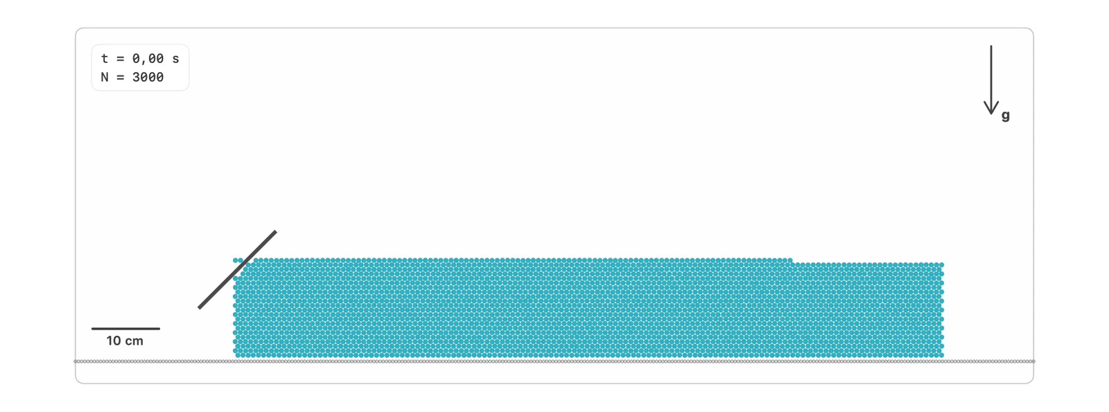
How do drag and lift forces scale for an inclined plate pushing a granular bed?
2D preset inspired by Percier et al. An inclined plate advances at constant speed over a settled bed and records boundary forces and mass in a measurement zone ahead of the plate.
- Parameters:
- Particles N · Mean diameter d · Polydispersity · Bed height · Plate length · Attack angle · Plow speed · Travel distance · Finite/periodic X condition
- Observables:
- F_D(t) · F_L(t) · M_zona(t) · F_D/(M_zona g) · F_L/(M_zona g) · mu_eff
- Study tools:
- Run Comparison not available · Parametric sweep
Model & numerical notes
- Use Prepare to settle the bed before activating the plow.
- Periodic-x mode is opt-in for long/headless runs.
- M_zone is a geometric estimate in an ahead-of-plate measurement window; it is not a physical boundary.
- The plow is a kinematic segment: plate degrees of freedom are not resolved.
Heap flow
How do surface avalanches and outflow develop when grains are continuously deposited onto an L-shaped heap?
Heap flow is an educational DEM preset inspired by the heap-flow surface geometry discussed by GDR MiDi. It uses a controlled particle source and an L-shaped cell to form a heap; grains discharge when they fall from the open right edge of the base. It is not a calibrated quantitative replica.
- Parameters:
- Mean diameter d · Active-particle limit N · L wall height H · L base length W · Base roughness diameter · Source width · Source x · Source height · Source-surface gap · Deposition rate · Friction μ
- Observables:
- Surface angle θ_surface(t) · Avalanche activity A(t) · Surface map h(x,t) · Discharged count N_out(t) · Mass flow rate Q_out(t) · Dimensionless 2D flow proxy Q*_2D(t) · Avalanche count and duration
- Study tools:
- Run Comparison · Parametric sweep
Model & numerical notes
- The source reuses inactive particle slots before appending new particles and respects a hard slot capacity.
- Discharged grains are detected after falling below the base at the open right edge; they are marked inactive and removed from contacts.
- The surface angle is fitted only when enough finite surface bins are available.
- Q*_2D is a 2D proxy Q_mass/(rho_2D d sqrt(gd)); it is not a calibrated Hele-Shaw flow rate.
- Force-network analysis is available but disabled by default.
Free-fall stream
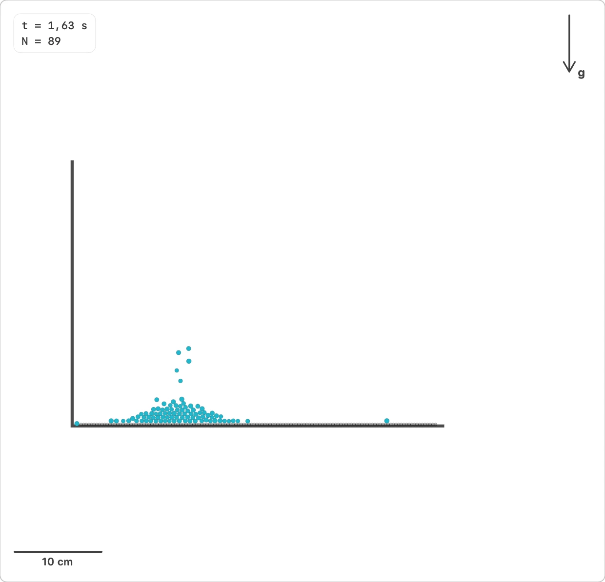
How do the center of mass and shape of a freely falling granular segment evolve when vacuum, uniform air and shielded drag are compared?
2D granular column without walls or cohesion. The visualization can follow the center of mass, while observables report fall, deformation, connectivity and geometric exposure to air.
- Parameters:
- Particles N · Mean diameter d · Polydispersity · Initial width D0 · Initial height L0 · External medium · Air damping γ_air · Shielding length · Laboratory/center-of-mass camera
- Observables:
- Y_cm(t) · V_cm(t) · A_cm(t) · Radius of gyration R_g(t) · Aspect ratio L_y/W_x · Instantaneous contacts and clusters · Mean exposure and drag force
- Study tools:
- Run Comparison not available · Parametric sweep
Model & numerical notes
- FF1 does not include cohesion: Royer et al. clustering remains for a later phase.
- Shielded air is a geometric model of differential drag, not CFD or capillary cohesion.
- The comoving camera is visual and does not change physical positions or velocities.
- Uniform linear air uses F_drag = -m γ_air v through ExternalMedium.
- There are no walls or floor; particles can fall indefinitely in the laboratory frame.
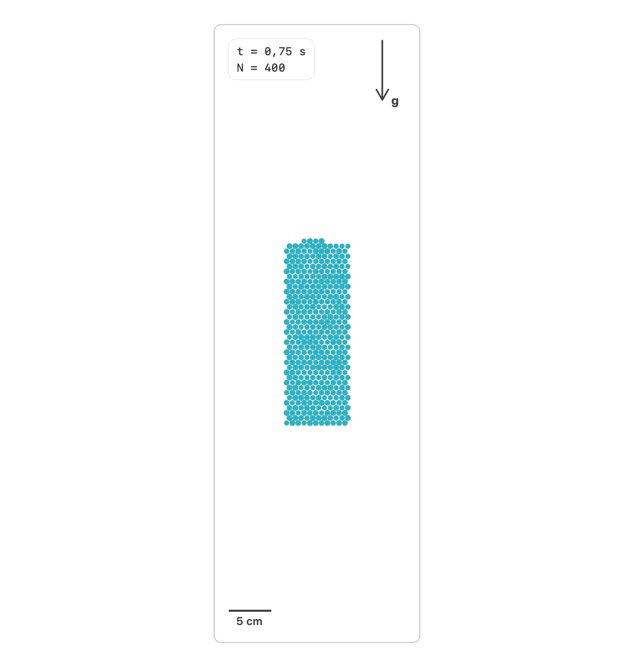
Intrusion and impact
Granular impact · 2D
How does a granular bed stop an intruder and transmit its momentum?
Prepare the bed, release the intruder, then compare penetration, downward speed and upward contact force. Recorded run calculates an independent recorded run for playback and export. This is a two-dimensional disk model, not a quantitative model of a sphere in 3D sand.
- Parameters:
- Number of bed grains · Reference grain diameter d · Projectile D/d and 2D density ratio · Launch speed (not contact speed) · Bed width / d · Friction, reference restitution and stiffness · Preparation seed
- Observables:
- Penetration below the initial bed surface · Projectile downward velocity · Upward resultant contact force · Contact network · Maximum overlap and kinetic energy
- Study tools:
- Run Comparison not available · Parametric sweep not available
Model & numerical notes
- SI units. Disk mass = density2D × πr²; moment of inertia = mr²/2. Density is in kg/m².
- Linear repulsive spring-dashpot contacts with tangential history and Coulomb friction; no extra macroscopic stopping force is added.
- Restitution calibrates an isolated pair of reference-sized grains. Effective restitution differs for walls, polydisperse grains and the projectile because their reduced masses differ.
- The projectile is excluded during bed preparation and inserted one grain diameter above the settled surface. Gravity increases its speed before first contact.
- The top is open; sidewalls and bottom are physical. Check sensitivity to bed width, depth, packing seed and timestep before interpreting scaling laws.
- Recorded run integrates contact-force impulse at every DEM step and stores interval means and peaks separately from video frames. Live plots and standard CSV are instantaneous samples.
- The impact preset opts into a small-grain cell grid with explicit large-disk queries. Other presets keep their default neighbor search.
- 5000 grains is an exploratory workload, not a convergence certificate. No air, cohesion, grain fracture or high-speed cratering physics.
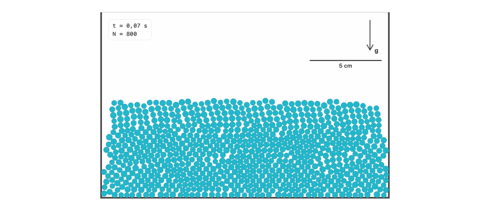
Deposition and piles
Angle of repose
How does an effective angle of repose emerge when grains are deposited from a localized source and form a pile?
Gravitational deposition on a rough base. Grains fall from a localized source and accumulate into a pile whose slope depends on friction, roughness and dissipation.
- Parameters:
- Particles N · Mean diameter d · Source width · Deposition height · Deposition rate · Base roughness · Gravity g · Friction μ · Global damping
- Observables:
- Pile height · Basal width · Estimated angle of repose · Kinetic energy · Contacts · delta max/R
- Study tools:
- Run Comparison not available · Parametric sweep
Model & numerical notes
- Deposit grains progressively from the source, without physical hopper walls.
- Adjust deposition rate to avoid severe initial overlaps.
- Monitor kinetic energy before measuring a stationary slope.
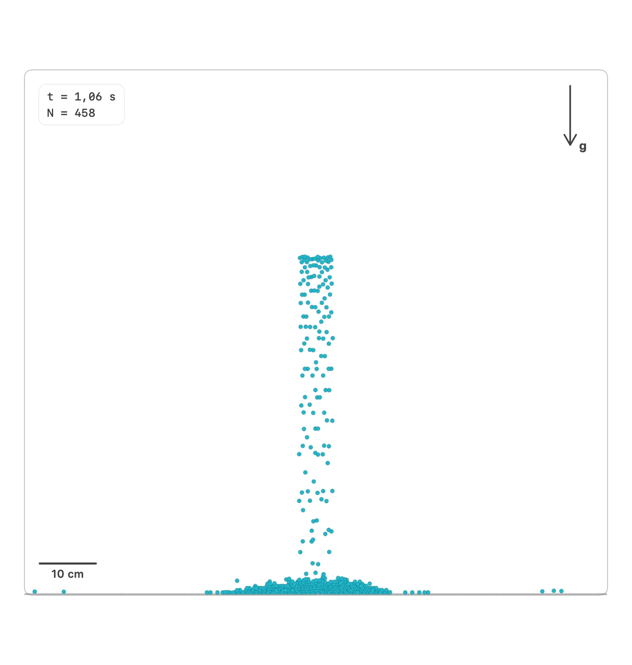
Granular pile
How does the basal load profile change when a granular pile is built by a localized source or by homogeneous rain?
2D granular pile inspired by the construction-history memory experiments of Vanel et al. The preset compares two initial conditions and measures the basal normal load with discrete sensors.
- Parameters:
- Construction mode · Particles N · Mean diameter d · Polydispersity · Basal width · Basal sensors · Friction μ
- Observables:
- q_y(x) [N/m] · q_y/(Mg/L) · Central dip index · F_base/Mg · Kinetic energy · Contacts
- Study tools:
- Run Comparison not available · Parametric sweep
Model & numerical notes
- Use Prepare to relax the pile before measurement.
- Basal load is reported as 2D line pressure in N/m.
- Source/rain comparisons are made in separate runs.
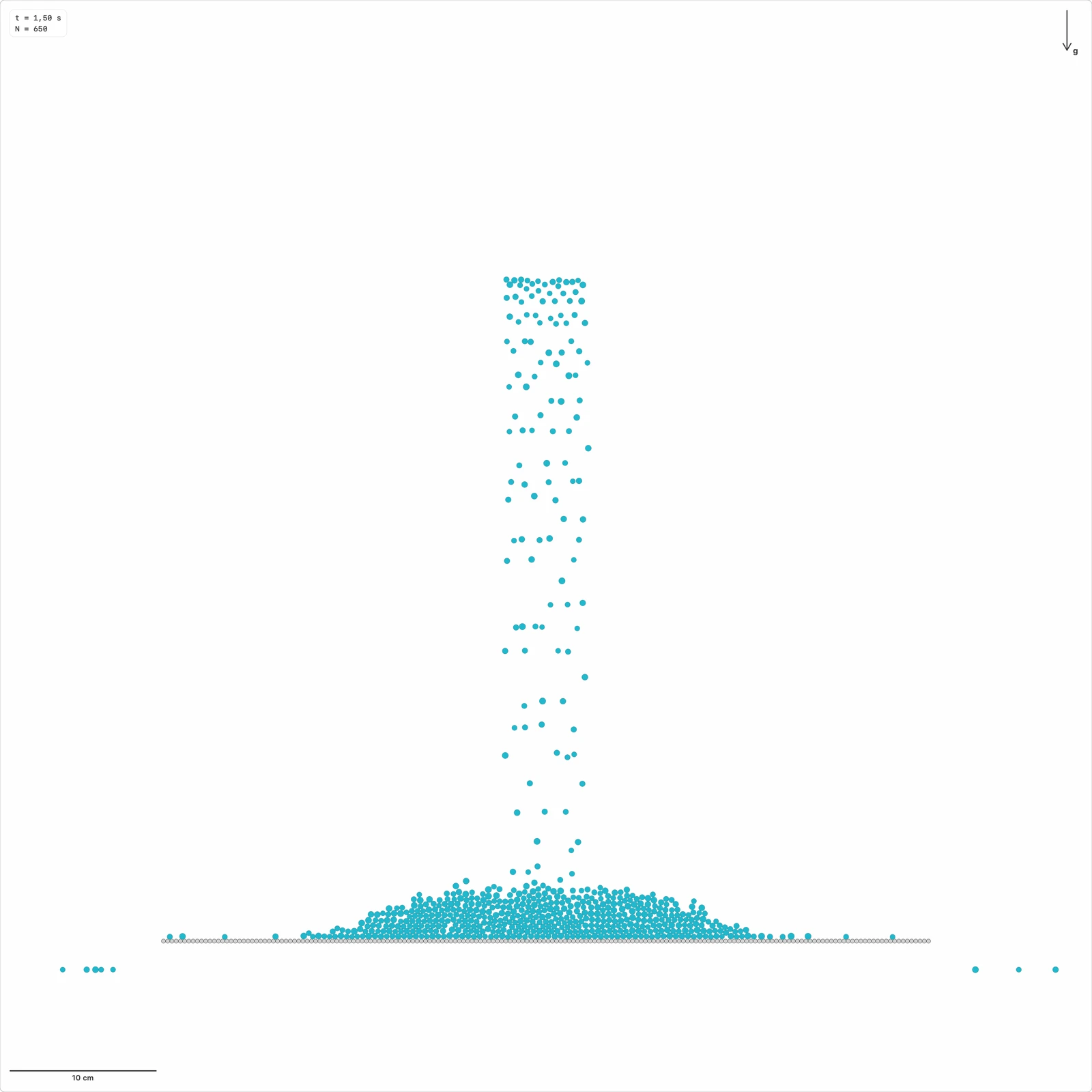
Granular avalanches
How does a pile respond to the addition of just one grain?
A reproducible disordered rough base with open ends. The next grain is released only after the entire pile has remained quiet, including particle rotation.
- Parameters:
- Additions · Grain diameter · Base width · Release height above base · Random gaps · Rest tolerance and duration
- Observables:
- Avalanche size S(n) · P(S), including S = 0 · Escaped grains · Relaxation time · Voronoi shape factor ζ
- Study tools:
- Run Comparison not available · Parametric sweep not available
Model & numerical notes
- 2D disk analogue; glass-plate friction and 3D sphere inertia are not represented. No power law is imposed.
- S counts old centres without a centre within d/7 in the next settled state. The new grain is excluded. ID displacement is reported separately.
- A timeout stops deposition; it never releases another grain into a moving pile.
- Voronoi is optional and evaluated only at rest. Cells touching the 4d local boundary and centres within 2d of the base are excluded; retained cells use exact half-plane clipping.
- The compact demo is not the paper geometry. The paper uses L = 600 mm, d = 4 mm, h = 280 mm and 55,000 additions. Its arXiv version excludes the first 4,500 events; configure the transient for your study.
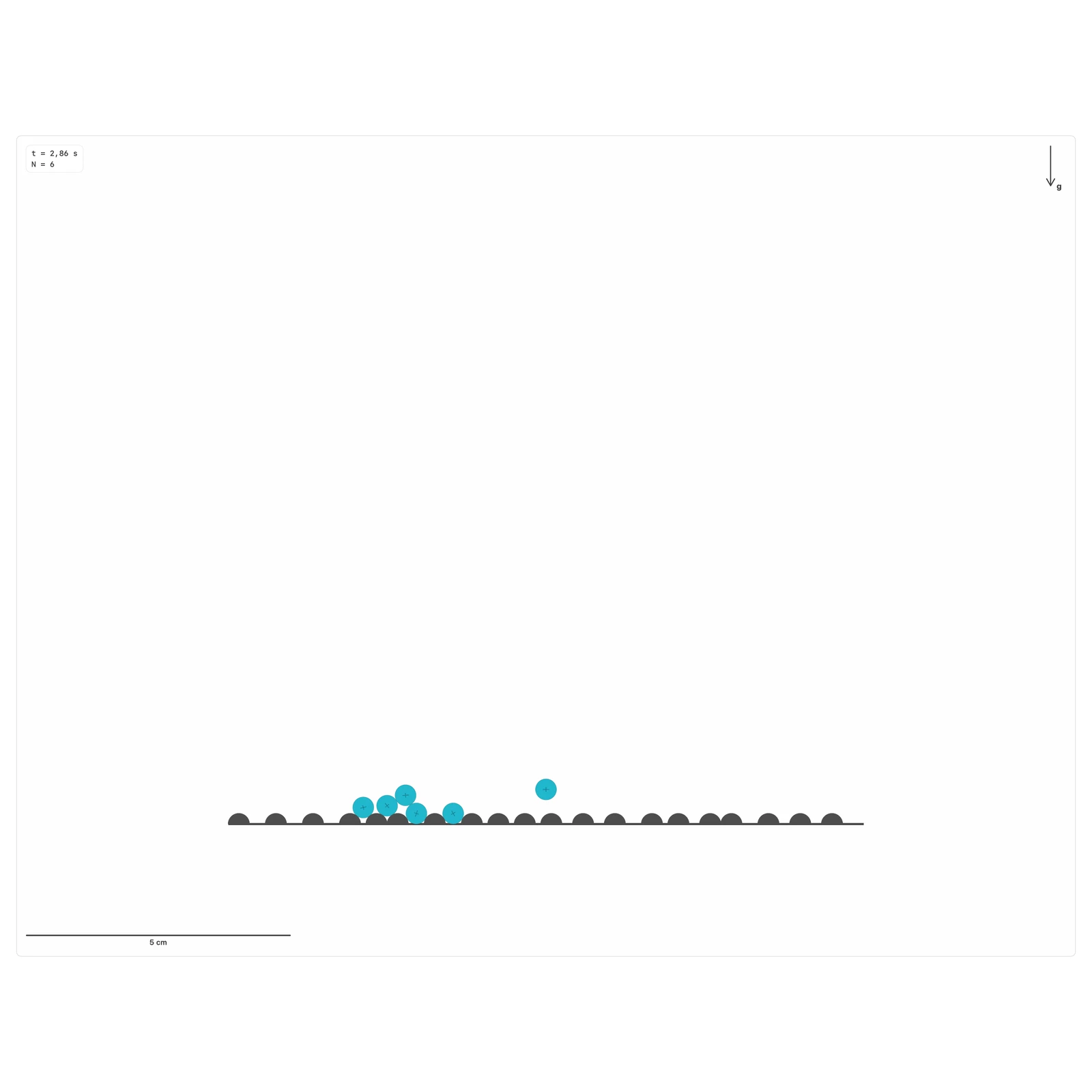
Curved-base deposition
How do pile shape and stability change when deposition occurs over a non-flat rough base?
Gravitational deposition from a localized source over a static rough boundary with flat, concave, convex or wavy geometry.
- Parameters:
- Base type · Base amplitude or curvature · Wavelength · Particles N · Mean diameter d · Source width · Source height or adaptive distance · Deposition rate · Base roughness
- Observables:
- Apparent angle of repose · Surface profile h(x) · h(x,t) map · Residual activity
- Study tools:
- Run Comparison · Parametric sweep
Model & numerical notes
- The base is a static DEM boundary made of segments and rough disks.
- The adaptive source only changes insertion position; it does not add forces.
- Control deposition rate and roughness to avoid initial overlaps.
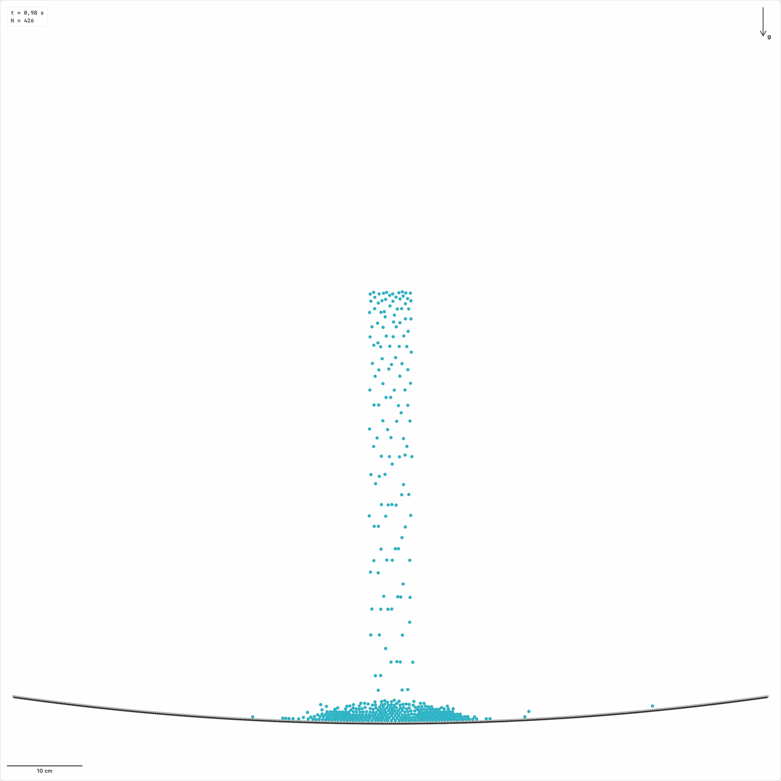
Segregation
Brazil nut
Under what conditions does a large intruder rise inside a vibrated granular bed?
Vibrated bed with a larger intruder particle. It supports studying segregation, percolation, convection and sensitivity to density and friction.
- Parameters:
- Small-grain radius · Intruder radius · Intruder density ρ · Initial height · Base agitation · Gravity g · Friction μ
- Observables:
- Intruder height · Kinetic energy · Contacts · Rise time · delta max/R
- Study tools:
- Run Comparison not available · Parametric sweep
Model & numerical notes
- Initialize the intruder without overlaps.
- Control agitation amplitude to avoid numerical ejection.
- Separate physical segregation from boundary effects.
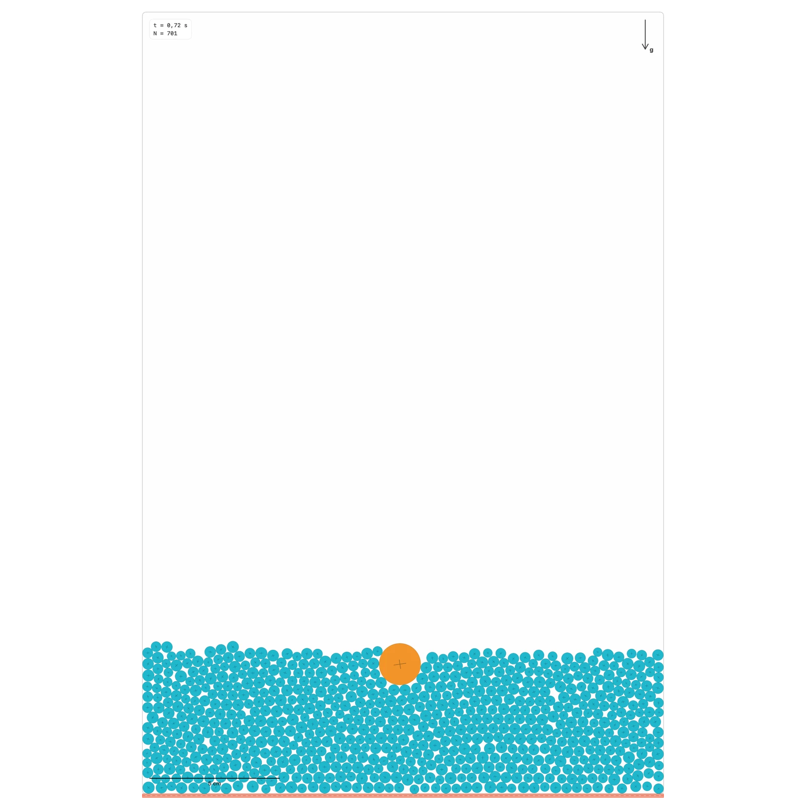
Granular mixing
How does mixing evolve between two initially separated granular populations?
Two granular species are placed initially separated inside a rotating drum. Rotation produces a surface active layer and a passive region that can mix or segregate particles depending on size, density, fill level and angular speed. This preset supports studying the competition between mixing and segregation.
- Parameters:
- Species fraction · Initial condition · RPM · Size ratio · Densities ρ_A/ρ_B · Friction μ · Drum radius · Gravity g · Roughness
- Observables:
- Mixing index M · Local concentration by species · Center of mass by species · Mean diameter by species · Kinetic energy · Granular activity
- Study tools:
- Run Comparison · Parametric sweep
Model & numerical notes
- Avoid initializations with overlaps.
- Ensure mass is consistent with density and radius.
- Use the mixing grid with a minimum number of particles per cell.
- Do not compute mixing if there are too few particles per bin.
- Throttle observables.
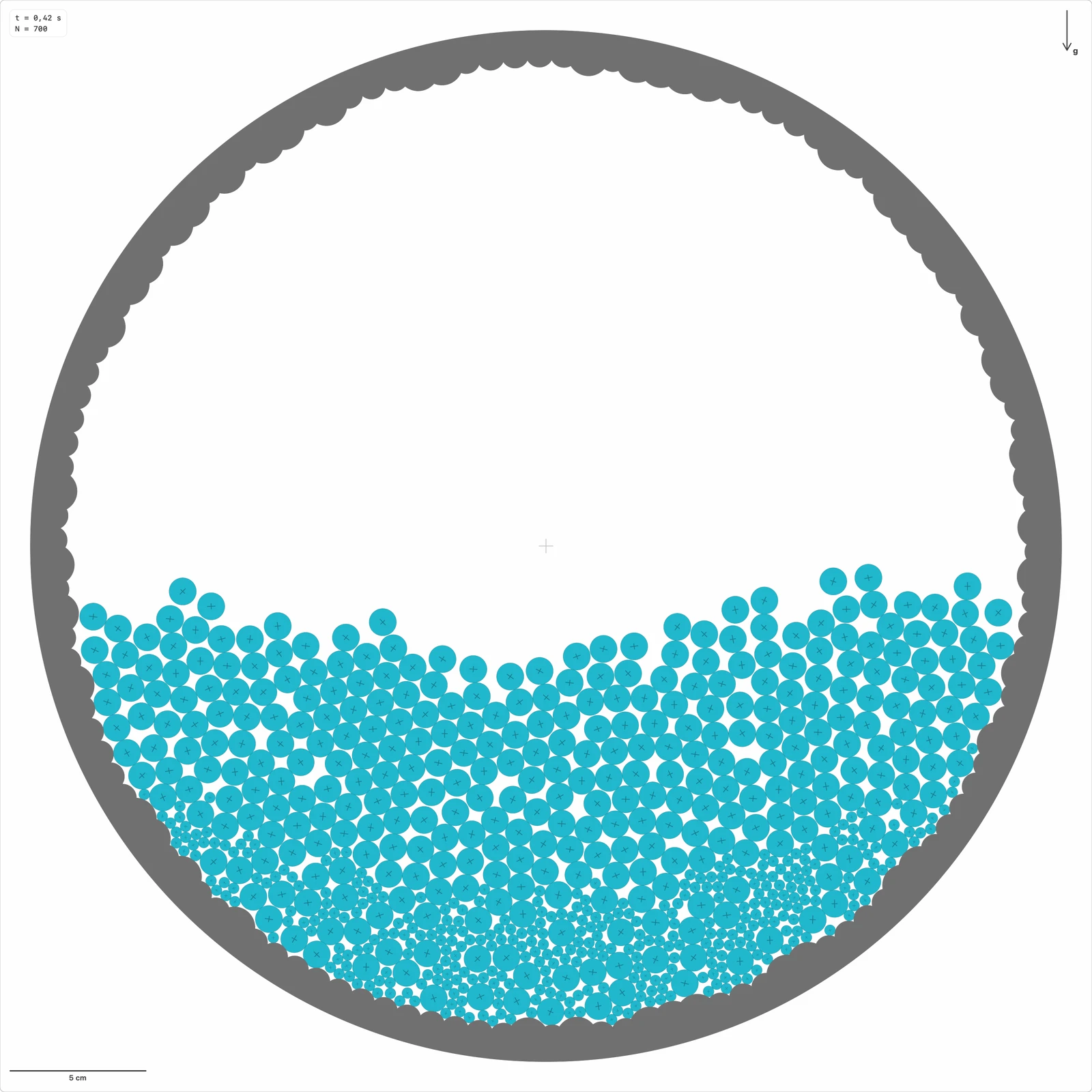
Forced / nonlinear dynamics
Simple bounce
How is the effective restitution of a particle bouncing on a rigid wall measured?
Minimal case of one particle under gravity colliding with a base. It validates potential/kinetic energy, normal damping and restitution measurement.
- Parameters:
- Teaching material · Radius · 2D density ρ · Initial height · Initial velocity · Normal restitution e_n · Friction μ
- Observables:
- Maximum height · Kinetic energy · Potential energy · Total energy · Effective restitution · Time between bounces
- Study tools:
- Run Comparison · Parametric sweep
Model & numerical notes
- Detect impact from the non-contact to contact transition.
- Use relative wall velocity if the wall moves.
- Monitor that energy decays when the impact is dissipative.
Vibrated base
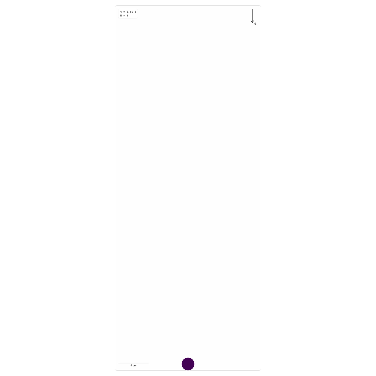
How do periodic orbits, subharmonics and chaos appear in a particle bouncing on a vibrating base?
A particle falls under gravity and collides with a vertically oscillating base. Energy is injected at each impact according to base phase and relative particle-wall velocity. Changing amplitude, frequency and restitution can produce periodic responses, period doubling and chaos.
- Parameters:
- Amplitude A · Frequency f · Gravity g · Normal restitution e_n · Friction μ · Initial height · Initial velocity · Mass/radius
- Observables:
- y(t) · vy(t) · Phase space vy vs y · Impact phase · Post-impact velocity vs phase · Maximum height · Time between bounces · Effective restitution
- Study tools:
- Run Comparison · Parametric sweep
Model & numerical notes
- Use relative particle-wall velocity.
- Detect impacts as a non-contact to contact transition.
- Phase phi = 2*pi*f*t mod 2*pi.
- Use circular buffers.
Vibrating ratchet
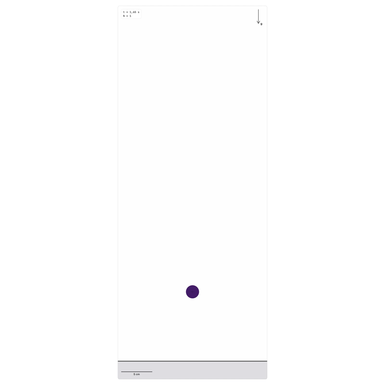
How can an asymmetric vibrating base rectify particle motion and produce lateral transport?
The preset explores how geometry, vibration intensity, forcing direction and particle size control activation, directional bias and mean lateral displacement. This version uses circular particles and supports vertical, horizontal or circular vibration with a 90-degree phase shift between x and y.
- Parameters:
- Tooth height h · Period w · Asymmetry length y · a = y/w · Number of teeth · Amplitude A · Frequency f · Forcing direction · Acceleration Γ · Particle radius · Friction μ and normal restitution e_n
- Observables:
- x(t) · y(t) · Delta x total · Intraperiod residual · Inter-tooth events · p_event · Directional bias · Drift velocity · Relative phase xi · Physical tooth jumps P(n_i) · Time-lag displacement and drift-corrected variance · Effective diffusion D_eff (single particle)
- Study tools:
- Run Comparison · Parametric sweep
Model & numerical notes
- Contact jumps use n_i = m_(i+1) - m_i with r in [y-w, y), not rounded displacement. The initial-tooth histogram is a separate diagnostic.
- Endpoints use DEM-step minima of height relative to the base with nearby ratchet contact; this differs from image-based y(t) minima in the experiment.
- Diffusion uses one particle, laboratory-frame unwrapped displacements and overlapping time origins at 50 Hz, retaining up to 900 s. The 2-20 s fit starts after 100 s and assumes stationary increments; D_eff is not a convergence claim.
- The linear DEM contact model and periodic trajectory are not a calibrated reproduction of the Hertzian LIGGGHTS draft or the finite-cell experiment.
- Domain width must be an exact multiple of period w.
- Lateral periodicity uses periodicXOnly and the tracker distinguishes wrapped position from accumulated displacement.
- The vibrating base must use relative particle-wall velocity.
- Horizontal and circular forcing move finite segments as a rigid body and resolve continuity with periodic copies.
- In circular mode, amplitude A is the base-trajectory radius and Γ is reported as A(2πf)^2/g.
Vibrated bed
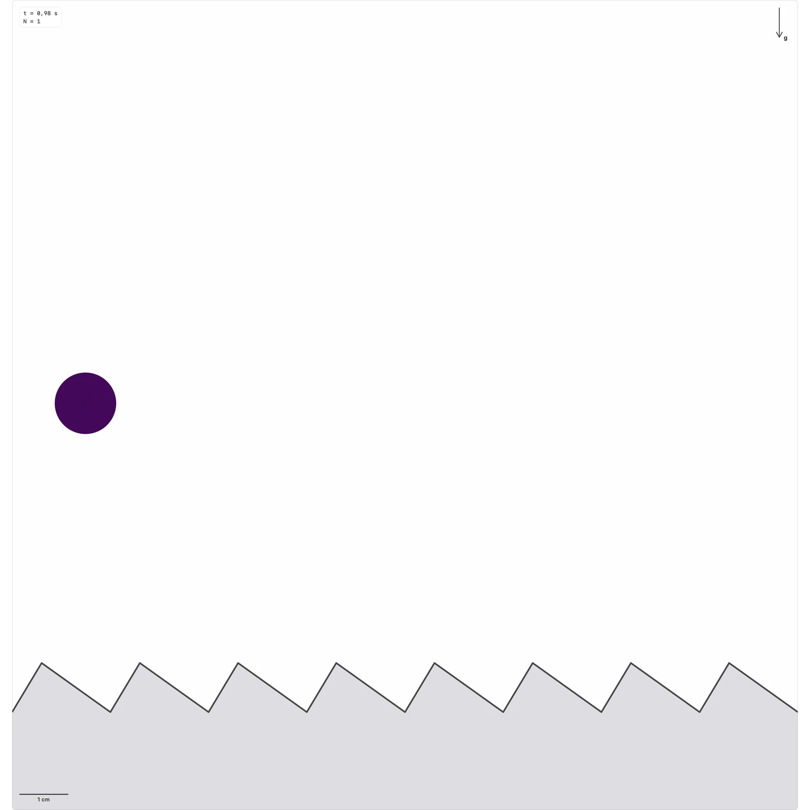
How does a granular bed fluidize when it receives energy from a vibrating base?
A vertically vibrated grain bed can show fluidization, compaction, saltation, convection and collective patterns. The key parameter is Γ, the maximum base acceleration normalized by gravity.
- Parameters:
- Particles N · Mean diameter d · Polydispersity · Amplitude A · Frequency f · Acceleration Γ = A(2πf)^2/g · Gravity g · Friction μ · Damping γ_n/γ_t
- Observables:
- Mean bed height · Vertical center of mass · Granular temperature · Kinetic energy · Airborne particle fraction · Contact count · Maximum overlap
- Study tools:
- Run Comparison · Parametric sweep
Model & numerical notes
- The moving base must use relative particle-wall velocity.
- Avoid an artificial elastic ceiling; the top remains open.
- Monitor stability when Γ is large.
- Use circular buffers for time observables.
- Stop or pause if NaN, high overlap or lateral particle loss appears.
Tapped compaction
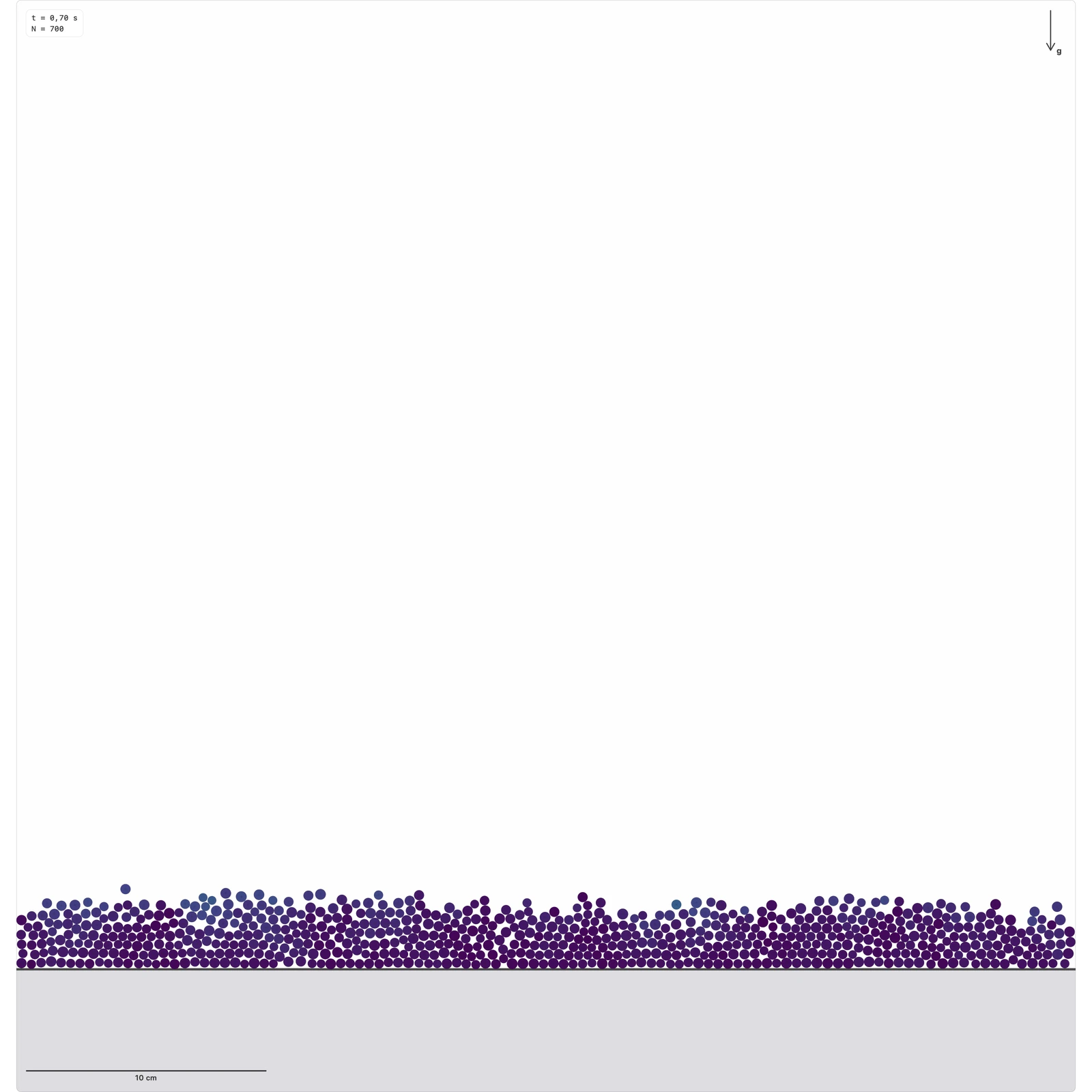
How does a gently deposited two-dimensional packing densify under repeated discrete taps separated by relaxation?
This preset is an educational two-dimensional soft-disk DEM adaptation of tapped-compaction experiments. Prepare deposits grains gradually under gravity and lets the bed relax before the first tap. The base and lateral walls then translate together during a raised-cosine pulse and remain still until the next tap. The reported packing fraction is nominal: the sum of disk areas divided by the rectangular bed envelope.
- Parameters:
- Particles N · Mean diameter d · Polydispersity · Peak cell rise A · Pulse frequency f · Tap period T · Peak acceleration Γ = 2π²Af²/g · Gravity g · Friction μ
- Observables:
- Settled nominal packing fraction φ_pile(n) · Bed height H_pile(n) · Granular temperature after each tap · Tap index n · Dimensionless acceleration Γ · Amplitude ratio A/d
- Study tools:
- Run Comparison not available · Parametric sweep
Model & numerical notes
- The raised-cosine pulse starts and ends with zero displacement and velocity, avoiding a discontinuous wall velocity.
- The default gentle tap uses A/d = 0.20 and Γ ≈ 1.45; limiting A/d alone does not limit acceleration when frequency increases.
- Colors follow initial horizontal bands. A fixed gray copy of the initial free surface is drawn behind the mobile grains; it has no mass, contacts or effect on observables.
- Prepare uses gradual gravity deposition followed by a rest stage; it is a reproducible 2D analogue rather than a literal nitrogen-fluidization replica.
- The tracker records one sample per tap during the rest interval, rather than sampling while the container is moving.
- φ_pile is a nominal 2D area fraction; soft-disk overlaps and boundary-layer corrections are not subtracted.
- This is a 2D educational model, not a quantitative reproduction of the original three-dimensional experiments.
- The inverse-log compaction law is useful as a phenomenological comparison, but it is not automatically fitted or asserted by this preset.
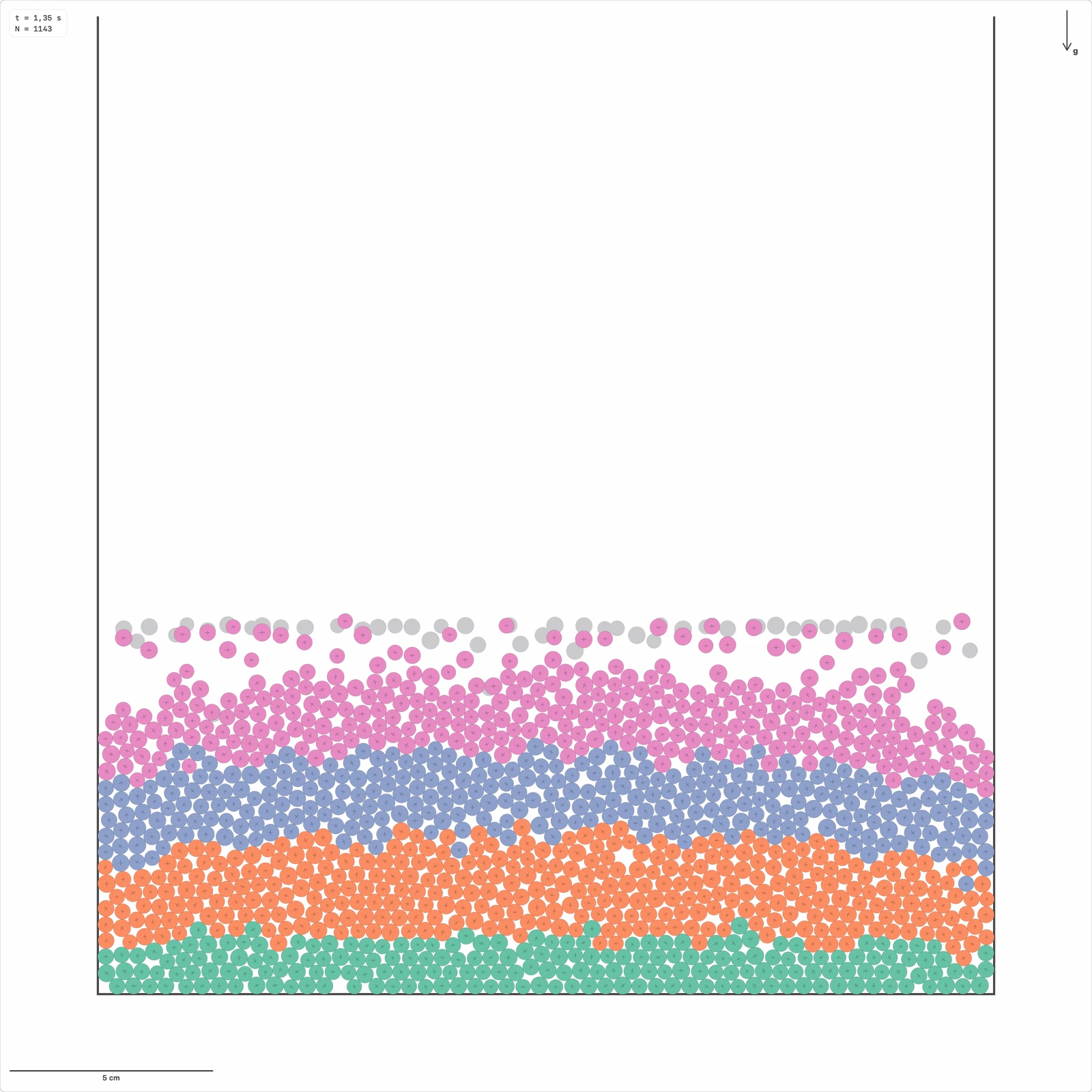
V-shaped bed
How does base geometry modify agitation, order and fluidization in a vibrated granular bed?
A grain bed is confined in a vertical cell whose V-shaped base vibrates sinusoidally. Changing the base angle breaks packing symmetry, which can promote defects, increase disorder and modify granular temperature at comparable injected energy.
- Parameters:
- Particles N · Mean diameter d · Polydispersity · Amplitude A · Frequency f · Acceleration Γ = A(2πf)^2/g · Gravity g · V-base angle · Friction μ · Damping γ_n/γ_t
- Observables:
- Acceleration Γ · Mean bed height · Vertical center of mass · Granular temperature · Kinetic energy · Flight fraction · Contact count · Velocity field · Maximum overlap
- Study tools:
- Run Comparison · Parametric sweep
Model & numerical notes
- The V-base moves as a rigid boundary with two synchronized inclined walls.
- Contacts with moving walls must use relative particle-wall velocity.
- Large angle changes rebuild the initial packing.
- Monitor high overlap, NaN and particles outside the domain.
- Topological observables such as psi6, defects and solid/fluid fraction remain future work.
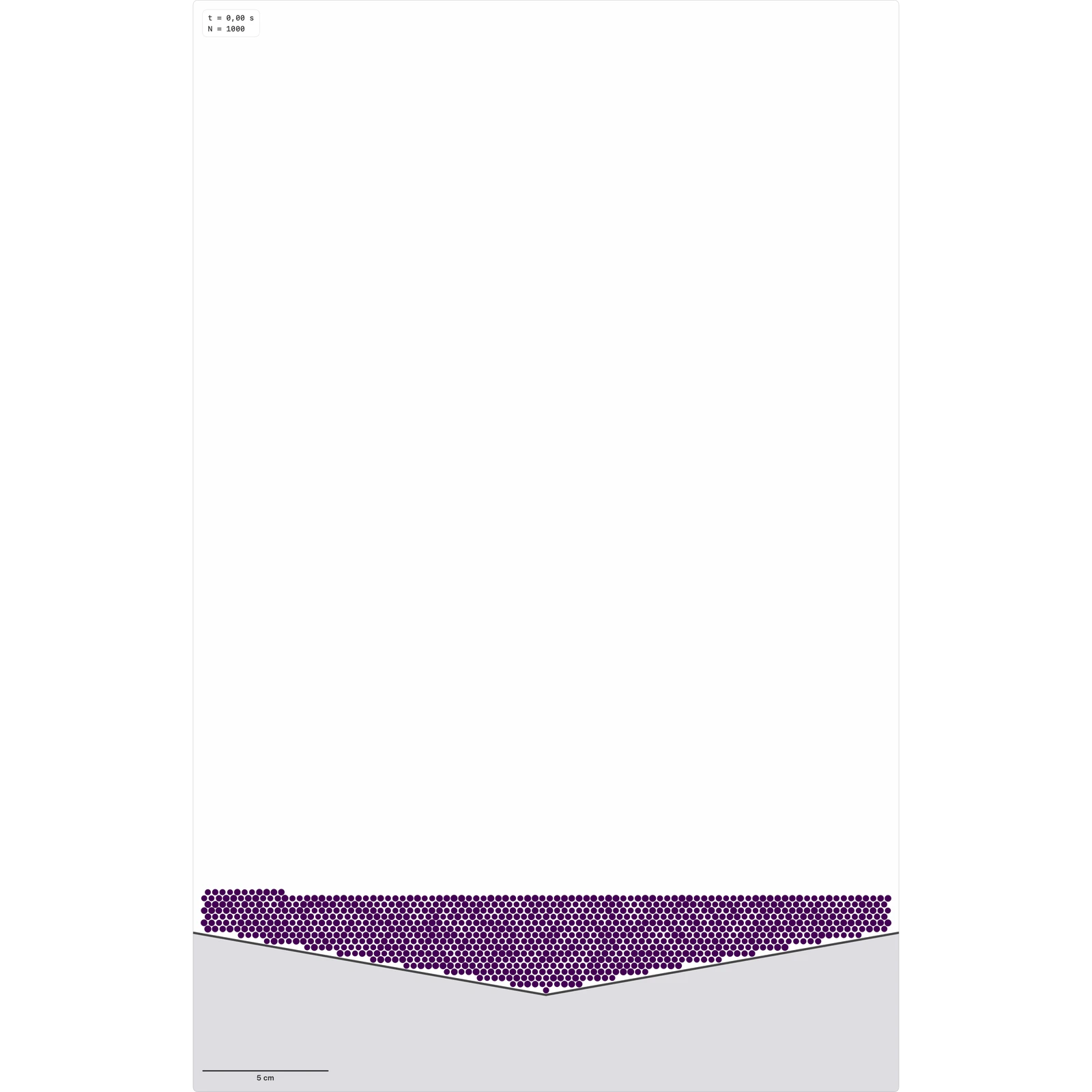
Vibrated quasi-2D layerExperimental
How do vertical confinement and vibration redistribute kinetic energy between horizontal and vertical motion in a shallow granular layer?
This exploratory preset uses an isolated three-dimensional sphere backend because projected particle overlap does not imply physical contact in a shallow cell. It is inspired by quasi-2D vibrated-layer experiments and is not yet a quantitatively calibrated reproduction.
- Parameters:
- Box width Lx · Box depth Ly · Gap ratio h/d · Particles N · Particle diameter d · Material density rho · Vibration amplitude A · Frequency f · Normal restitution · Normal stiffness
- Observables:
- Mean vertical position · Vertical layer occupancy · Horizontal granular temperature Txy · Vertical granular temperature Tz · Anisotropy Tz/Txy · Top and bottom wall contacts
- Study tools:
- Run Comparison not available · Parametric sweep not available
Model & numerical notes
- The MVP uses normal spring-dashpot contacts only; tangential history and friction are future work.
- Projected overlaps are allowed visually and never create contacts by themselves.
- A and f are primary controls; Gamma and A/d are derived.
- N is the primary population control; projected filling fraction is derived.
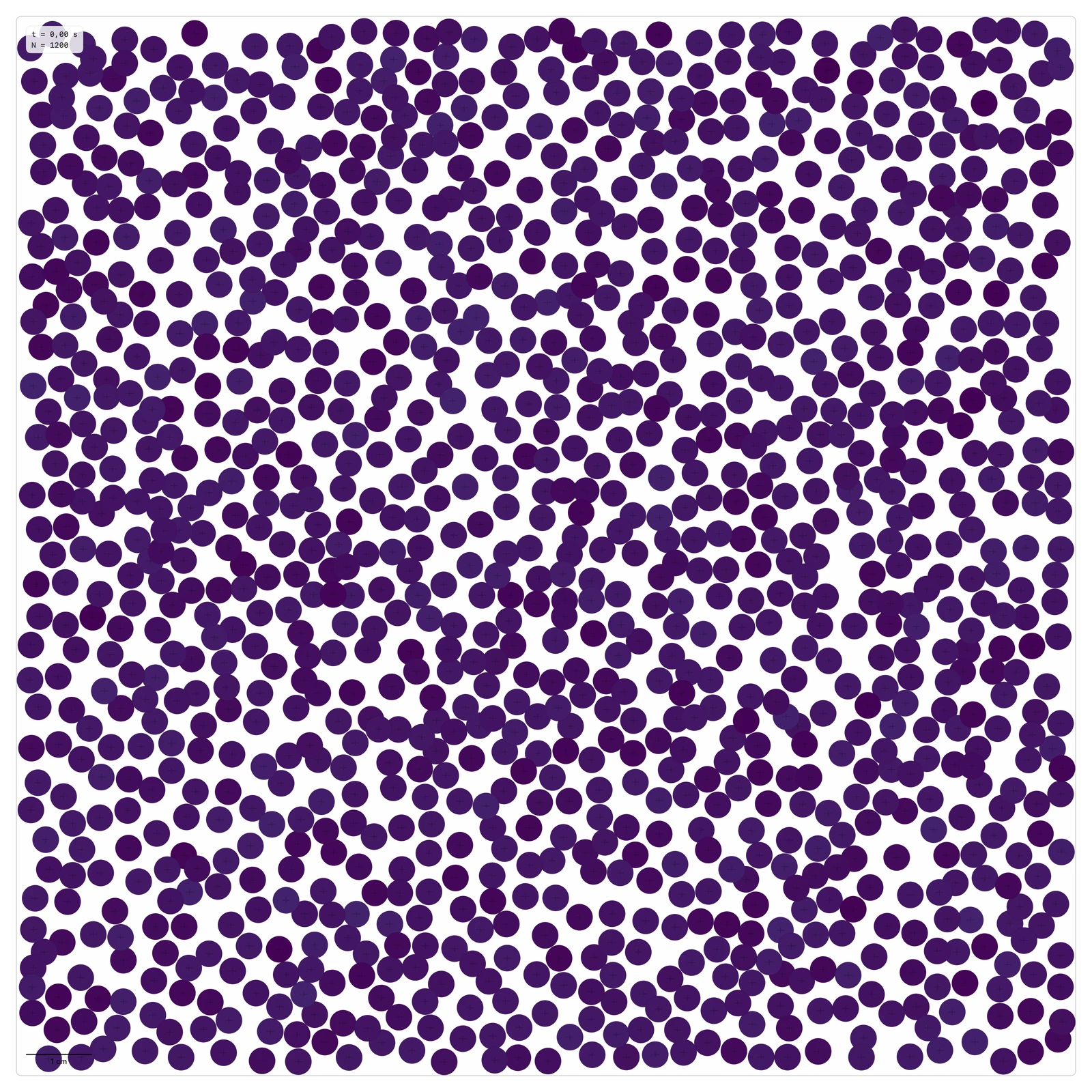
Granular Brownian motionExperimental
When does a large tracer on a vibrated granular layer exhibit horizontal diffusion?
Contacts drive the tracer without added random forces. The initial transient is excluded from statistics. Mass and inertia follow solid-sphere geometry; at equal density the default 3d tracer (4.5 mm) has 27 times the bath-grain mass. A Brownian regime is not guaranteed.
- Parameters:
- Bath N and d · Tracer D/d and density ratio · A and f · Friction and restitution · Transient and sampling interval
- Observables:
- Drift-centered horizontal MSD versus lag · Horizontal velocity correlation · Tracer height · Unwrapped trajectory
- Study tools:
- Run Comparison not available · Parametric sweep not available
Model & numerical notes
- SI units; CPU/Double/Velocity Verlet. Check overlap and dt/2 convergence.
- Positions are in the moving-base frame; horizontal coordinates are unwrapped for statistics.
- Multiple overlapping time origins are correlated. Repeat seeds and box sizes before interpreting diffusivity.
- Background observables include tracer.csv and diffusion.csv; particle dumps remain optional.
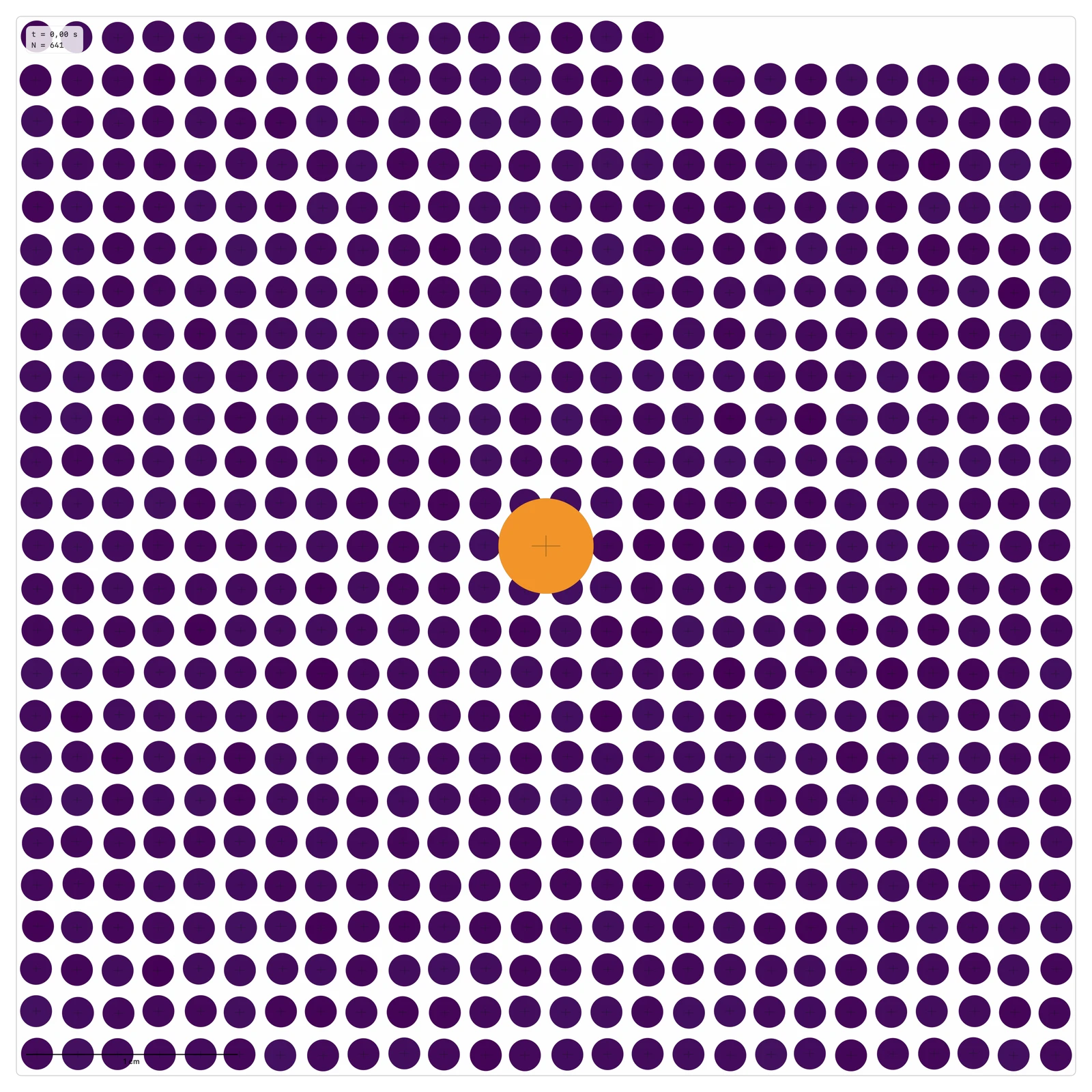
Rotating drum
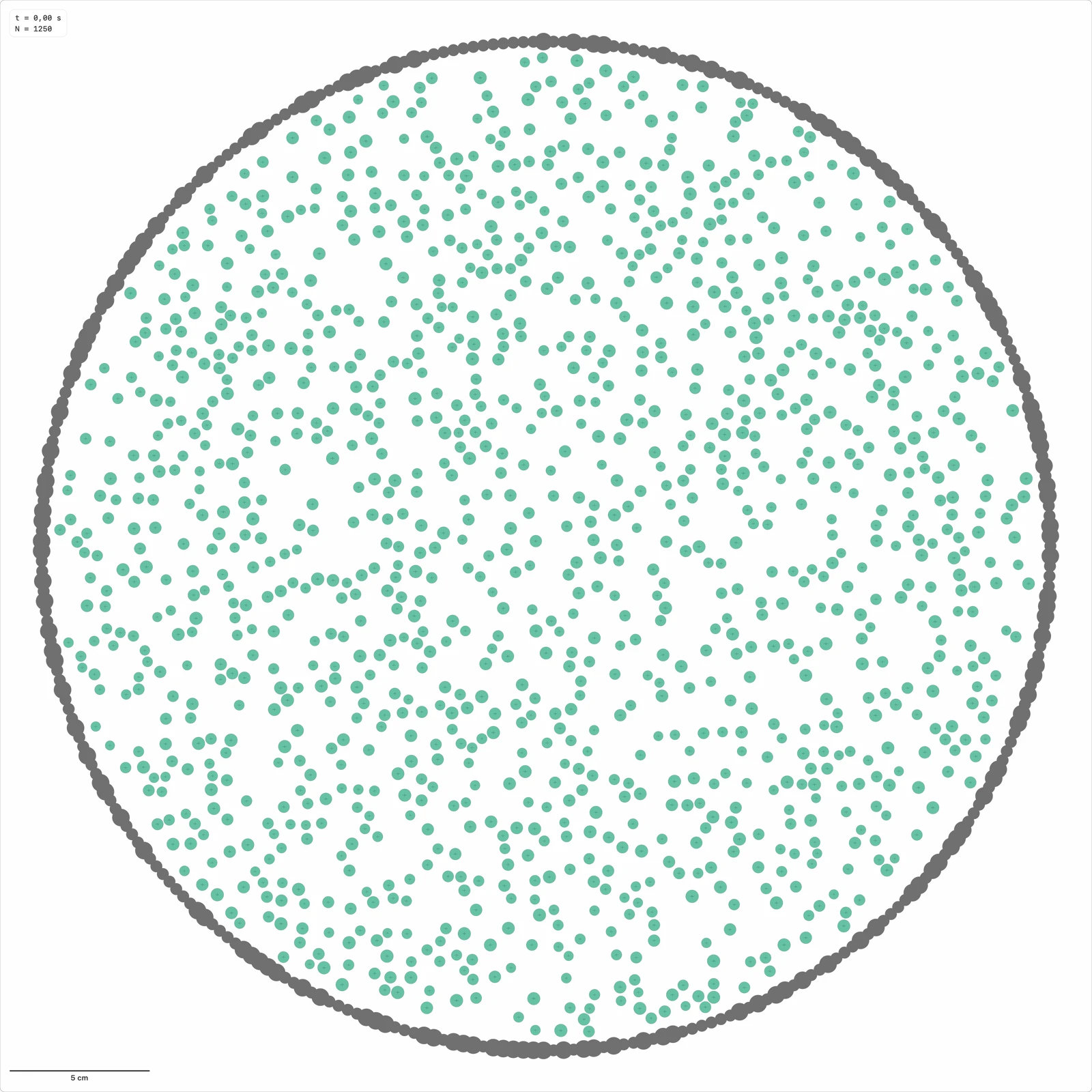
How do surface avalanches form in a granular material inside a slowly rotating drum?
A set of grains is confined in a circular drum rotating under gravity. At low rotation speeds, the material can remain nearly solid until the free surface reaches a critical angle and an avalanche occurs. Increasing rotation speed can move the system from intermittent avalanches to continuous flow.
- Parameters:
- Particles N · Grain size · Polydispersity · Drum radius · Angular speed in rpm · Grain-grain friction μ · Grain-wall friction μ · Gravity g · Wall roughness
- Observables:
- Center-of-mass angle · Free-surface angle · Minimum and maximum angles · Kinetic energy · Avalanche frequency · Granular activity · Contact count · Force chains and synthetic photoelasticity
- Study tools:
- Run Comparison · Parametric sweep
Model & numerical notes
- Use relative velocity with the rotating wall.
- Avoid initial overlaps.
- Monitor particles outside the domain.
- Use circular buffers for charts.
- Enable photoelasticity only when contacts/forces need to be inspected, because it captures extra samples.
- Detect avalanches from energy peaks or rapid changes in surface angle.
- TODO: estimate theta_surface, theta_min and theta_max with a robust free surface.
Shear and compaction
Granular stick-slip
When does spring-driven granular friction produce intermittent slip instead of smooth motion?
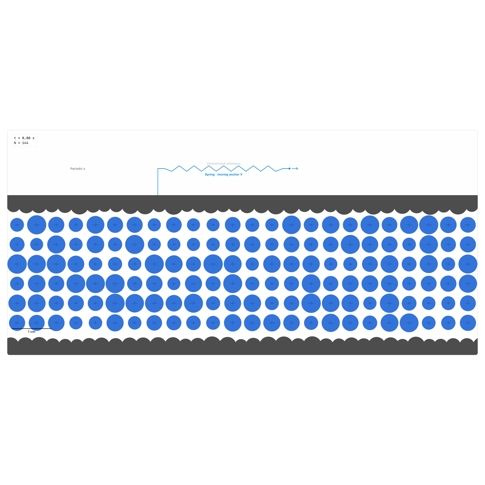
Prepare a polydisperse bed under a constant normal load, then drive the spring anchor at constant speed. The guided upper plate responds dynamically to the spring and the grains, and can rise as the layer dilates. Loading and slip emerge from frictional DEM contacts; the plate velocity is not prescribed.
- Parameters:
- Drive speed V [m/s] · Drive stiffness k [N/m] · Total normal load W [N] · Plate mass M [kg] · Grain friction μ · Initial layers, columns and mean diameter [m] · Disordered or regular rough surfaces; random seed
- Observables:
- Spring force and contact resistance [N] · Plate velocity and drive speed [m/s] · Dilation from prepared height [mm] · Grain, plate and spring energy [J]
- Study tools:
- Run Comparison · Parametric sweep
Model & numerical notes
- A 2D educational analogue inspired by Nasuno et al.; its parameters are not calibrated to reproduce the 3D experiment quantitatively.
- The layer is periodic horizontally, with a fixed rough base. The upper boundary is a non-rotating inertial body covered by glued disks. Its unwrapped displacement drives the spring extension.
- Disordered surfaces have independently seeded radii (±20%) and nonuniform spacing. Glued boundary disks overlap to close the surface, including the periodic seam; only the complete domain repeats. Regular surfaces remain available for comparison.
- Two or three initial layers represent a strongly confined granular interface. Layer thickness can change the frictional response, so a thin bed is not a quantitative substitute for a deeper sample. Width is columns × 1.22 × mean diameter; adjust columns and diameter together to keep width fixed.
- M*ẍ = k*(V*t−x) + F_contact,x. M*ÿ = F_contact,y − W. W is the complete applied normal force (including any weight), independent of the inertial mass control. Grain gravity is 9.81 m/s².
- Normal linear spring–dashpot contacts and tangential history with a Coulomb cap are the existing DEM law. No bulk static/dynamic friction switch is imposed. Polydispersity is ±20% in radius.
- Prepare settles with the spring anchor held and additional damping. Contact history and spring preload are retained. The experimental clock and dilation reference start after preparation; damping is then removed. Resetting a physical control requires a new preparation.
- Spring force and instantaneous contact resistance differ during plate acceleration. The energy chart separates plate/grain kinetic energy and spring storage; it is not a closed-system energy balance.
- Plate height is the nominal gap between the inward envelope planes of the actual rough surfaces, not a spatially averaged local aperture. Dilation measures vertical plate displacement from the prepared state.
- Intermittency and smooth sliding depend on speed, stiffness, load, packing and transient duration; no universal transition speed is claimed. Check overlap and convergence when changing the time step.
Simple shear cell
How do contacts and stress anisotropies organize during granular shear?
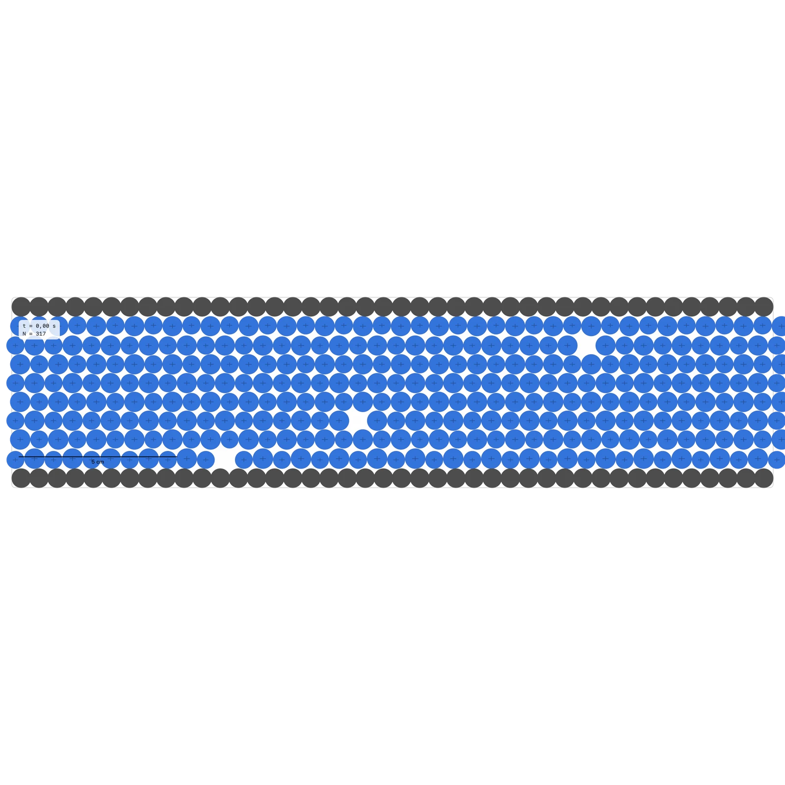
Rectangular simple-shear cell at fixed height. A grain band is confined between a fixed rough lower wall and a rough upper wall that moves horizontally; synthetic photoelasticity is an optional Analysis layer.
- Parameters:
- Number of grains · Mean diameter d · Particle-size distribution and polydispersity · Target area fraction phi · Packing method · Top-wall speed · Ramp time · Friction μ · Normal stiffness k_n / k_t/k_n ratio · Photoelastic sensitivity
- Observables:
- Shear strain gamma and strain rate · Tangential and normal 2D wall stress [N/m] · Effective friction |tau|/sigma_n · Profile vx(y) · Solid fraction phi(y) · Coordination Z and fabric anisotropy · Optional force chains and synthetic fringes
- Study tools:
- Run Comparison not available · Parametric sweep
Model & numerical notes
- Cell height is fixed; compression-positive stresses assume unit out-of-plane thickness.
- Top and bottom roughness are fixed to avoid geometric coupling with dMean.
- Use periodicity only in x.
- The default size-aware triangular lattice inserts the requested population whenever the available site capacity permits; use Prepare to relax this reproducible initial state before shear.
- The bidisperse option uses a discrete 50:50 number mixture with exact dL/dS = 1.40 through the structured initializer. It is a reproducible ordered initial condition, not a direct sample of a random steady state.
- Activate the top wall with a smooth ramp.
- Monitor overlaps near roughness.
Biaxial compression
How does a dense granular packing develop strength and dilatancy under axial compression at controlled lateral stress?
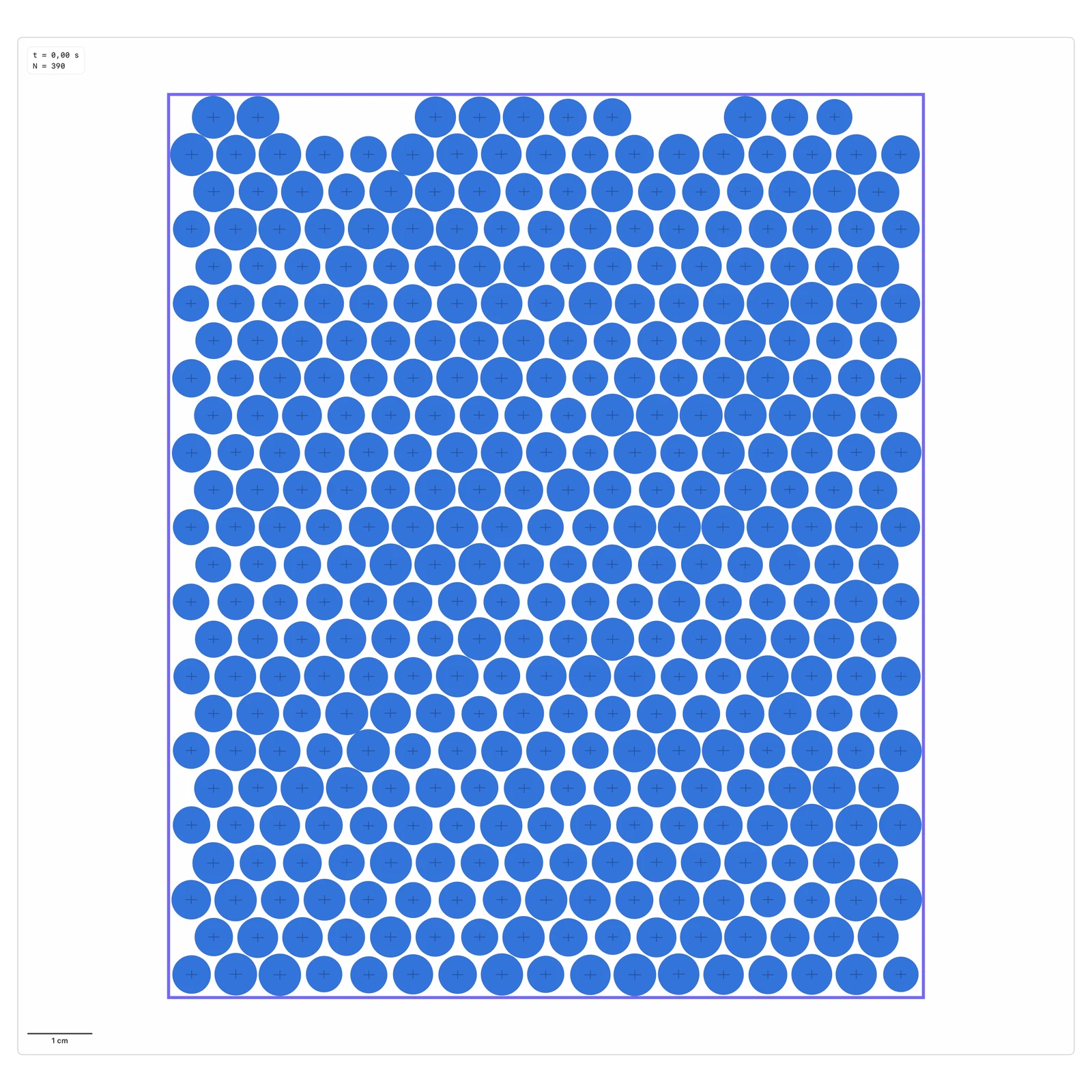
A centered specimen is enclosed by four fitted walls, prepared isotropically to p0, then compressed vertically at prescribed strain rate while a bounded wall servo maintains sigma3 near p0.
- Parameters:
- Preparation pressure p0 [N/m] · Axial strain rate [1/s] · Lateral servo gain [m2/(N s)] · Maximum servo speed [m/s] · Friction and contact stiffness
- Observables:
- q/p versus axial strain · Volumetric strain and dilatancy · Packing fraction phi · Coordination Z · Fabric anisotropy · Maximum overlap
- Study tools:
- Run Comparison not available · Parametric sweep
Model & numerical notes
- Compression is positive and stresses are 2D line loads in N/m for unit thickness.
- The preparation servo remains active during relaxation and requires both pressure and kinetic-energy stability before axial loading.
- Indigo wall lines show the instantaneous cell; arrows identify walls that are moving.
- The lateral controller is proportional, speed-limited and paused above the overlap guardrail.
- The preset stops at the declared maximum axial strain.
Isotropic compaction
How do pressure, coordination and fabric evolve as a soft-disk assembly approaches jamming?
Four fitted planar walls advance symmetrically at equal strain rate in small increments; each increment is followed by kinetic-energy relaxation before compression resumes.
- Parameters:
- Target packing fraction phi · Wall speed [m/s] · Strain increment · Relaxation energy threshold [J/particle] · Friction and contact stiffness
- Observables:
- p(phi) [N/m] · Z(phi) · Fabric anisotropy · Maximum overlap · Kinetic and contact energy
- Study tools:
- Run Comparison not available · Parametric sweep
Model & numerical notes
- The four walls remain symmetric and the geometric center is invariant.
- The default target phi = 0.84 crosses the expected 2D soft-disk jamming region; lower targets may correctly finish with negligible pressure.
- Indigo wall lines show the instantaneous cell; arrows identify walls that are moving.
- Wall motion pauses when the overlap guardrail is exceeded.
- Bulk modulus estimates require enough relaxed p(phi) samples and are not inferred from a single increment.
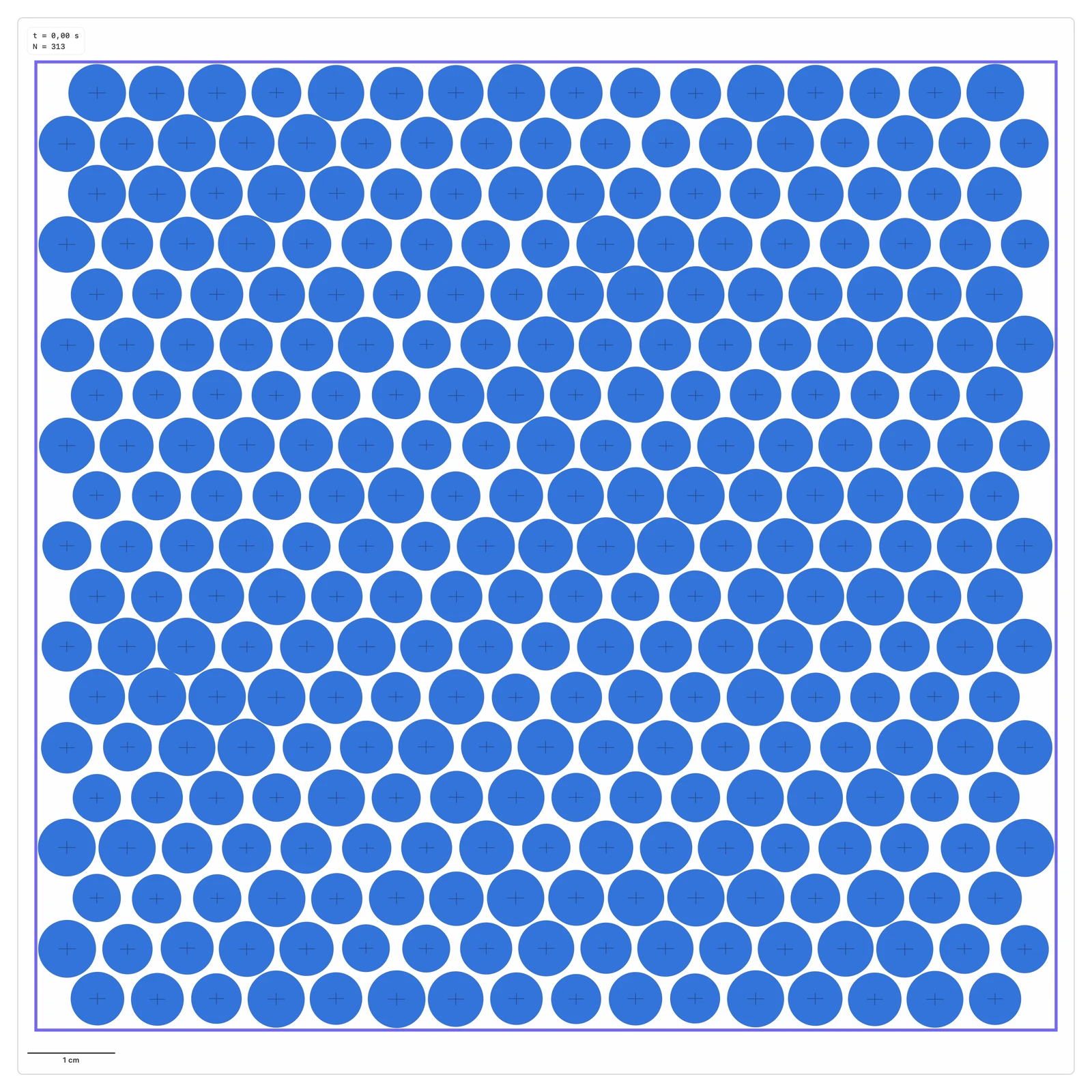
Periodic isotropic jamming
How do coordination, force residual and contact-force statistics evolve during quasi-static isotropic compression toward jamming?
A periodic polydisperse soft-disk packing is compressed affinely in small isotropic increments and relaxed after every increment until a force-residual criterion is met.
- Parameters:
- Particles N and mean radius r · Target area fraction φ_target · Compression increment strain Δε · Force-residual tolerance R_F · Maximum relaxation steps · Friction μ and stiffness ratio k_t/k_n · Deterministic seed
- Observables:
- Packing fraction φ · Force residual R_F · Coordination number Z · Mean overlap ratio · P(f_n/<f_n>) and its moments · P(|f_t|/<|f_t|>) · Coulomb mobilization P(η)
- Study tools:
- Run Comparison not available · Parametric sweep
Model & numerical notes
- Both directions are periodic; gravity and physical walls are absent.
- Compression is affine and alternates with force relaxation, rather than moving four walls.
- Success requires the target φ and final R_F tolerance; safety or iteration limits terminate with a reported failure reason.
- R_F is dimensionless and must be interpreted together with maximum overlap and finite-state diagnostics.
- The preset is a finite educational analogue of Boberski et al.; the reference study used approximately 14,200 disks.
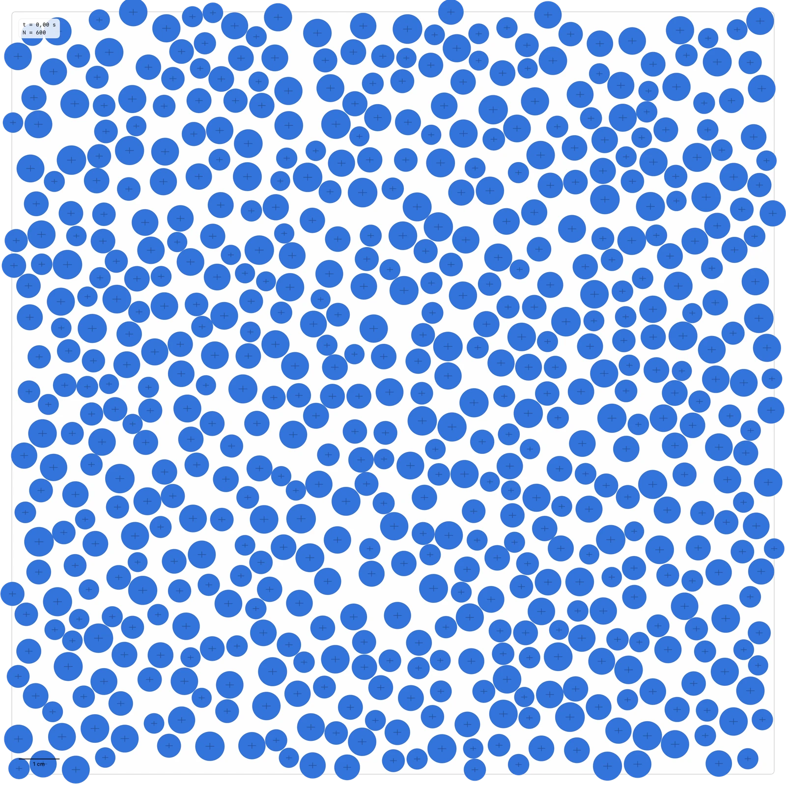
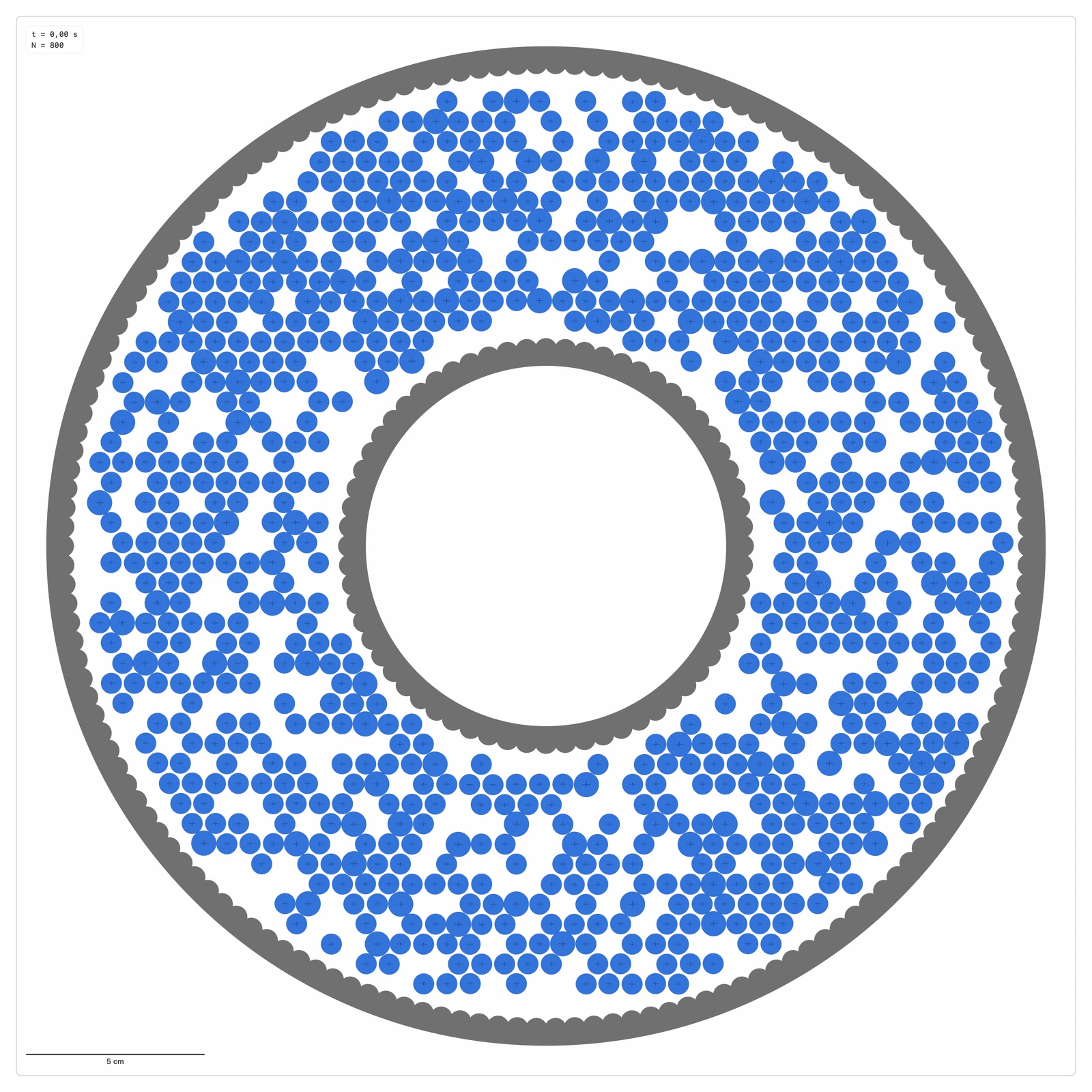
Couette cell
How does a dense annular packing reach a reproducible steady shear state before velocity and force statistics are measured?
A rough-wall annular Couette cell with an exploratory mode and a Howell et al. (1999) validation mode using a quasi-static drive and an explicit preshear protocol.
- Parameters:
- Inner radius R_i · Outer radius R_o · Particles N · Mean diameter d · Polydispersity · Angular speed Ω · Study mode and preshear rotations · Friction μ · Normal stiffness k_n / k_t/k_n ratio
- Observables:
- Radial profile v_theta(r) · Inner/outer wall contacts · Kinetic energy · Maximum overlap · Particles inside the annulus · Clearance against rough walls · Preshear progress and stationarity · P(f_n/<f_n>), P(|f_t|/<|f_t|>) and P(η)
- Study tools:
- Run Comparison not available · Parametric sweep
Model & numerical notes
- C1 uses wall disks as rough boundaries, not smooth circular walls.
- The inner wall uses RotatingFixedDisk2D drivers paired by ID with real disks.
- The outer wall remains fixed.
- Packing uses reproducible polar rejection and validates overlap against real wall disks.
- Howell mode uses the published bidisperse geometry and quasi-static angular-speed range as a validation reference.
- Its preshear stationarity criterion is an operational DEM criterion; the experimental optical force proxy G² is not identified with a single contact force.
Keep exploring.
Granular LAB 2.1 for Mac. Works offline. No account required.
Read the user manual (PDF)
Cite Granular LAB
Varas, G. Granular LAB: a native macOS workspace for granular and active-matter simulations. Version 2.1.0, 2026.
Apple, the Apple logo, Mac, and macOS are trademarks of Apple Inc., registered in the U.S. and other countries. App Store is a service mark of Apple Inc.